Accessibility in practice

Author

Emmanouil Tranos

Published

November 30, 2023

Setup

To run this pratical you need to have an RStudio project as discussed in the previous practical.

library(tidyverse)
library(accessibility)
library(sf)
library(kableExtra)
library(rprojroot)
library(osrm)

path <- find_rstudio_root_file()

# This is the project path
knitr::opts_chunk$set(include=TRUE, message=FALSE, warning=FALSE)

Aims of the practical

The aim of this practical is to calculate different accessibility indicators. For a brief overview about accessibility, please have a look at (Rodrigue 2020) (for example here ). For in depth reviews have a look at Holl (2007), El-Geneidy and Levinson (2022) and Shi et al. (2020) as well as at some older and well-cited papers such as Geurs and Van Wee (2004) and Bruinsma and Rietveld (1998). The below typology of accessibility concepts is from Holl (2007).

Network access
- distance to access the network
- travel opportunities
Travel cost measures
- network access + distance/time travelled on the network
Market potential accessibility
- destinations at greater distance provide diminishing opportunities
- $Acc_i = \sum_j\frac{W_j} {c_{ij}^a}$

Among other R packages, the practical is based on the accessibility package. Some of the below materials are based on the package’s vignette.

Let’s start with using the toy data that comes with the accessibility package. As you can see below, the data comes in R’s native data format called .Rds and, therefore, we use the relevant function to read it – readRDS().

The first data object we are using is the travel time matrix between all potential origins and destinations in city of Belo Horizonte, Brazil. As you can see, the matrix is stored in a long format and not as an $n*n$ matrix. If you check the dimension of that object you will understand what I mean (dim(travel_matrix)).

data_dir <- system.file("extdata", package = "accessibility")

travel_matrix <- readRDS(file.path(data_dir, "travel_matrix.rds")) 

head(travel_matrix)

           from_id           to_id travel_time
1: 89a88cdb57bffff 89a88cdb57bffff         5.8
2: 89a88cdb57bffff 89a88cdb597ffff        47.0
3: 89a88cdb57bffff 89a88cdb5b3ffff        48.0
4: 89a88cdb57bffff 89a88cdb5cfffff        47.0
5: 89a88cdb57bffff 89a88cd909bffff        64.0
6: 89a88cdb57bffff 89a88cd90b7ffff        59.0

Then, we are loading the characteristics of each location. As you can see, the id records match with the from_id and to_id from the travel_matrix.

land_use_data <- readRDS(file.path(data_dir, "land_use_data.rds"))
head(land_use_data)

                id population jobs schools income_per_capita income_decile
1: 89a881a5a2bffff        381  180       0           22369.1            10
2: 89a881a5a2fffff        269  134       0            3205.1             9
3: 89a881a5a67ffff        929  143       0           11394.0            10
4: 89a881a5a6bffff        249   61       0            3659.8             9
5: 89a881a5a6fffff        176   11       0            4905.1            10
6: 89a881a5b03ffff        681 1071       0            2200.2             8

The first accessibility function we are using is cost_to_closest(). As per its name, it calculates the minimum travel cost to the closest n number of opportunities. In our example, as travel cost we understand the travel time between origins and destinations included in the column travel_time from the travel_matrix object. We are only interested in the closest (n=1) opportunity, which in this example is a school.

mtc <- cost_to_closest(
  travel_matrix,
  land_use_data,
  opportunity = "schools",
  travel_cost = "travel_time",
  n = 1
)

head(mtc)

                id travel_time
1: 89a881a5a2bffff          29
2: 89a881a5a2fffff          24
3: 89a881a5a67ffff          28
4: 89a881a5a6bffff          33
5: 89a881a5a6fffff          32
6: 89a881a5b03ffff          17

The next measure is the total number of opportunities (in other words, the cumulative opportunities) within a cut-off of the travel cost. So, the below provides the number of jobs accessible within 30 minutes of travel time.

cum_cutoff <- cumulative_cutoff(
  travel_matrix,
  land_use_data,
  opportunity = "jobs",
  travel_cost = "travel_time",
  cutoff = 30
)

head(cum_cutoff)

                id  jobs
1: 89a881a5a2bffff 14561
2: 89a881a5a2fffff 29452
3: 89a881a5a67ffff 16647
4: 89a881a5a6bffff 10700
5: 89a881a5a6fffff  6669
6: 89a881a5b03ffff 37029

If the above was a form of active accessibility – that is how many opportunities one can access from their location – the below offers a passive form of accessibility – that is how many individuals can be reached from each destination within a cuttof. The latter is based on travel_time in the below.

passive_cum_cutoff <- cumulative_cutoff(
  travel_matrix,
  land_use_data,
  opportunity = "population",
  travel_cost = "travel_time",
  cutoff = 30,
  active = FALSE
)

head(passive_cum_cutoff)

                id population
1: 89a881a5a2bffff      11053
2: 89a881a5a2fffff      31903
3: 89a881a5a67ffff      12488
4: 89a881a5a6bffff      14474
5: 89a881a5a6fffff      15053
6: 89a881a5b03ffff      69582

Last, but not least we can calculate the gravity-based accessibility indicators, or, in other words, potential accessibility indicators. This is the same measure as the example we discussed during the class. The intuition is that the furthest away each opportunity is, the less important it becomes. So, the accessibility of a location $i$ is equal to the sum of all opportunities available divided – in other words discounted – by the distance or the cost to reach them. The negative_exp function can take different decay functions (see here). We know from previous studies that the exponential function represents better shorter interactions (e.g. within cities) while the power function works better for longer distance interactions (e.g. migrations flows) Oshan (2021).

$Acc_{i} = \sum_j \frac{W_j}{d_{ij}^2}$

negative_exp <- gravity(
  travel_matrix,
  land_use_data,
  opportunity = "schools",
  travel_cost = "travel_time",
  decay_function = decay_exponential(decay_value = 0.2)
)

head(negative_exp)

                id    schools
1: 89a88cdb57bffff 0.03041853
2: 89a88cdb597ffff 1.15549493
3: 89a88cdb5b3ffff 0.56519126
4: 89a88cdb5cfffff 0.19852152
5: 89a88cd909bffff 0.41378042
6: 89a88cd90b7ffff 0.95737555

And now we can plot these metrics. The grid object is a toy spatial dataset of the places we calculate the above accessibility indicators. We first load these spatial data, merge them with the acessibility indicator we want to plot and then we plot these data.

grid <- system.file("extdata/grid_bho.rds", package = "accessibility")
grid <- readRDS(grid)

spatial_data <- merge(grid, cum_cutoff, by = "id")

ggplot() +
  geom_sf(data = spatial_data, aes(fill = jobs), color = NA) +
  labs(
    title = "Job accessibility by transit in under 30 min.",
    fill = "Accessible jobs"
  ) +
  scale_fill_viridis_c() +
  theme_void()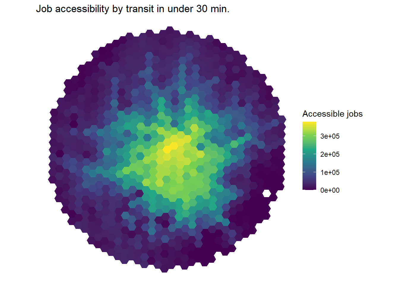

London example

All the above were based on the data that came together with the accessibility package. Let’s repeat this exercise using some real world data from data.london.gov.uk. Jobs and population per Local Authority represent the opportunities.

jobs <- read_csv("https://data.london.gov.uk/download/jobs-and-job-density-borough/79e85749-e38d-4bb6-8327-c60c6be27222/Jobs_and_Job_Density.csv") %>% 
  filter(year == 2020) %>%  # I am only using 2020 data. Remove this line 
                            # to see what will happen to the data.
  glimpse()

Rows: 49
Columns: 5
$ code           <chr> "E09000001", "E09000002", "E09000003", "E09000004", "E0…
$ area           <chr> "City of London", "Barking and Dagenham", "Barnet", "Be…
$ year           <dbl> 2020, 2020, 2020, 2020, 2020, 2020, 2020, 2020, 2020, 2…
$ number_of_jobs <dbl> 630000, 71000, 163000, 85000, 149000, 129000, 391000, 1…
$ job_density    <dbl> 83.73, 0.52, 0.64, 0.54, 0.69, 0.62, 1.98, 0.58, 0.72, …

pop <- read_csv("https://data.london.gov.uk/download/land-area-and-population-density-ward-and-borough/77e9257d-ad9d-47aa-aeed-59a00741f301/housing-density-borough.csv") %>% 
  filter(Year == 2020) %>% # This is a projection, but it will work for now
  glimpse()

Rows: 36
Columns: 10
$ Code                            <chr> "E09000001", "E09000002", "E09000003",…
$ Name                            <chr> "City of London", "Barking and Dagenha…
$ Year                            <dbl> 2020, 2020, 2020, 2020, 2020, 2020, 20…
$ Source                          <chr> "GLA Population Projections", "GLA Pop…
$ Population                      <dbl> 8046, 218367, 407148, 254970, 343853, …
$ `Inland_Area _Hectares`         <dbl> 290.4, 3610.8, 8674.8, 6058.1, 4323.3,…
$ Total_Area_Hectares             <dbl> 314.9, 3779.9, 8674.8, 6428.6, 4323.3,…
$ Population_per_hectare          <dbl> 27.7, 60.5, 46.9, 42.1, 79.5, 22.4, 11…
$ Square_Kilometres               <dbl> 2.9, 36.1, 86.7, 60.6, 43.2, 150.1, 21…
$ Population_per_square_kilometre <dbl> 2770.7, 6047.6, 4693.4, 4208.8, 7953.6…

Jobs and pop include observations for spatial units other than London’s 33 Local Authorities. Explore pop and jobs to see that. Therefore, we use the inner_join() function to join them. See here how it works. You should be able to understand the different functions to join data.

df <- inner_join(jobs, pop, by = c("code" = "Code")) %>% 
  filter(area != "London") %>% 
  rename(id = code)

To produce a nicer looking table I am using here the kableExtra package. It just adds some nice styling for html outputs.

df %>% kbl() %>%
  kable_styling(full_width = F) %>%   #Nice(r) table
  scroll_box(width = "900px", height = "400px")

id	area	year	number_of_jobs	job_density	Name	Year	Source	Population	Inland_Area _Hectares	Total_Area_Hectares	Population_per_hectare	Square_Kilometres	Population_per_square_kilometre
E09000001	City of London	2020	630000	83.73	City of London	2020	GLA Population Projections	8046	290.4	314.9	27.7	2.9	2770.7
E09000002	Barking and Dagenham	2020	71000	0.52	Barking and Dagenham	2020	GLA Population Projections	218367	3610.8	3779.9	60.5	36.1	6047.6
E09000003	Barnet	2020	163000	0.64	Barnet	2020	GLA Population Projections	407148	8674.8	8674.8	46.9	86.7	4693.4
E09000004	Bexley	2020	85000	0.54	Bexley	2020	GLA Population Projections	254970	6058.1	6428.6	42.1	60.6	4208.8
E09000005	Brent	2020	149000	0.69	Brent	2020	GLA Population Projections	343853	4323.3	4323.3	79.5	43.2	7953.6
E09000006	Bromley	2020	129000	0.62	Bromley	2020	GLA Population Projections	336395	15013.5	15013.5	22.4	150.1	2240.6
E09000007	Camden	2020	391000	1.98	Camden	2020	GLA Population Projections	257384	2178.9	2178.9	118.1	21.8	11812.4
E09000008	Croydon	2020	144000	0.58	Croydon	2020	GLA Population Projections	400272	8650.4	8650.4	46.3	86.5	4627.2
E09000009	Ealing	2020	160000	0.72	Ealing	2020	GLA Population Projections	361833	5554.4	5554.4	65.1	55.5	6514.3
E09000010	Enfield	2020	126000	0.59	Enfield	2020	GLA Population Projections	342993	8083.2	8220.1	42.4	80.8	4243.3
E09000011	Greenwich	2020	102000	0.52	Greenwich	2020	GLA Population Projections	292466	4733.4	5043.9	61.8	47.3	6178.8
E09000012	Hackney	2020	152000	0.76	Hackney	2020	GLA Population Projections	289488	1904.9	1904.9	152.0	19.0	15197.0
E09000013	Hammersmith and Fulham	2020	165000	1.28	Hammersmith and Fulham	2020	GLA Population Projections	190721	1639.7	1715.4	116.3	16.4	11631.1
E09000014	Haringey	2020	94000	0.51	Haringey	2020	GLA Population Projections	288913	2959.8	2959.8	97.6	29.6	9761.1
E09000015	Harrow	2020	90000	0.57	Harrow	2020	GLA Population Projections	261348	5046.3	5046.3	51.8	50.5	5179.0
E09000016	Havering	2020	95000	0.59	Havering	2020	GLA Population Projections	261830	11235.0	11445.7	23.3	112.3	2330.5
E09000017	Hillingdon	2020	206000	1.03	Hillingdon	2020	GLA Population Projections	316253	11570.1	11570.1	27.3	115.7	2733.4
E09000018	Hounslow	2020	169000	0.95	Hounslow	2020	GLA Population Projections	284358	5597.8	5658.5	50.8	56.0	5079.8
E09000019	Islington	2020	247000	1.32	Islington	2020	GLA Population Projections	242827	1485.7	1485.7	163.4	14.9	16344.7
E09000020	Kensington and Chelsea	2020	149000	1.41	Kensington and Chelsea	2020	GLA Population Projections	160794	1212.4	1238.4	132.6	12.1	13262.4
E09000021	Kingston upon Thames	2020	89000	0.76	Kingston upon Thames	2020	GLA Population Projections	182728	3726.1	3726.1	49.0	37.3	4904.0
E09000022	Lambeth	2020	175000	0.73	Lambeth	2020	GLA Population Projections	340324	2681.0	2724.9	126.9	26.8	12693.9
E09000023	Lewisham	2020	84000	0.39	Lewisham	2020	GLA Population Projections	317465	3514.9	3532.0	90.3	35.1	9031.9
E09000024	Merton	2020	97000	0.71	Merton	2020	GLA Population Projections	212658	3762.5	3762.5	56.5	37.6	5652.1
E09000025	Newham	2020	136000	0.55	Newham	2020	GLA Population Projections	363552	3619.8	3857.4	100.4	36.2	10043.3
E09000026	Redbridge	2020	90000	0.46	Redbridge	2020	GLA Population Projections	312264	5641.9	5644.2	55.3	56.4	5534.7
E09000027	Richmond upon Thames	2020	100000	0.80	Richmond upon Thames	2020	GLA Population Projections	201713	5740.7	5876.1	35.1	57.4	3513.7
E09000028	Southwark	2020	310000	1.34	Southwark	2020	GLA Population Projections	330290	2886.2	2991.3	114.4	28.9	11443.8
E09000029	Sutton	2020	82000	0.63	Sutton	2020	GLA Population Projections	211297	4384.7	4384.7	48.2	43.8	4819.0
E09000030	Tower Hamlets	2020	321000	1.32	Tower Hamlets	2020	GLA Population Projections	328043	1978.1	2157.9	165.8	19.8	16583.5
E09000031	Waltham Forest	2020	85000	0.46	Waltham Forest	2020	GLA Population Projections	290024	3880.8	3880.8	74.7	38.8	7473.3
E09000032	Wandsworth	2020	147000	0.62	Wandsworth	2020	GLA Population Projections	332731	3426.4	3522.0	97.1	34.3	9710.8
E09000033	Westminster	2020	747000	3.93	Westminster	2020	GLA Population Projections	259981	2148.7	2203.0	121.0	21.5	12099.5

Next, we are bringing the spatial data – that is the polygons – for London’s Local Authorities. We start by downloading all the polygons for all Local Authorities in the country. Please go to this webpage, download the geojson file and save it to the appropriate data folder within your project directory.

However, we don’t need all the Local Authorities, but instead we only need to ones within London. Therefore we use the filter option to select only the Local Authorities which are included within – this is the %in% operator – the df$id column. Finally, we create a new object which only includes the centroids of these polygons. Why are we doing this? Because we need to calculate distances and accessibility metrics for specific points and we will use these points as representative for each Local Authority.

Tip

Do you see any problems with this approach?

path.shape <- paste0(path, "/data/Local_Authority_Districts_(May_2021)_UK_BFE.geojson")

london <- st_read(path.shape) %>%
  dplyr::filter(LAD21CD %in% (df$id))

Reading layer `LAD_MAY_2021_UK_BFE_V2' from data source 
  `C:\Users\nw19521\OneDrive - University of Bristol\Bristol\teaching\urban_analytics_city_science\data\Local_Authority_Districts_(May_2021)_UK_BFE.geojson' 
  using driver `GeoJSON'
Simple feature collection with 374 features and 9 fields
Geometry type: MULTIPOLYGON
Dimension:     XY
Bounding box:  xmin: -8.649996 ymin: 49.86463 xmax: 1.768937 ymax: 60.86087
Geodetic CRS:  WGS 84

london.centres <- st_centroid(london)

Now we need to actually calculate the distance matrix. We are going to use a real world road network to perform what is known as routing. There is a great discussion about routing and before you move forward I would encourage you to read the relevant section from Lovelace, Nowosad, and Muenchow (2019), which can be found here.

We are using the osmr package which can do routing for us. The details of the osrm package can be founf here.

The below code creates a distance table between all the london.centres. We are interested in distance measured as time – i.e. duration – by car. The osrm package offers other options too.

dist <- osrmTable(loc = london.centres, 
                  measure = "duration",
                  osrm.profile = "car")

The output of the above is a list with an $n*n$ distance matrix, and a dataframe with the longitude and latitude of the origins and destinations. We are mostly interested in the former, so we start the data wrangling by creating a help dataframe with these distances, or in other words, durations. We then add row and column names using the london.centres names. We can just do that because the matrix follows the same order as the intimal spatial data of Local Authorities. I always like to throw in a dim function just to keep an eye on the dimensions of the objects I create. Indeed, the dist object is a $33*33$ matrix as it should have been.

Then, we need to convert the $n*n$ matrix to a long format. If you remember, we used to call this format an edge list. There are different way to do this. We can use the ready-made function odmatrix_to_od() from the od package. To see how it works, make sure that the od package is installed and then type the following: od::odmatrix_to_od. This will reveal how the odmatrix_to_od() function works under the hood. As you can see the magic happens by using the following R-base function: as.data.frame(as.table(odmatrix)). Therefore, I just used the below R-base function. You can, of course, use directly the odmatrix_to_od() function.

help <- dist$durations 

rownames(help) <- as.vector(london.centres$LAD21CD)
colnames(help) <- as.vector(london.centres$LAD21CD)

dim(dist$durations)

[1] 33 33

dist.df <- as.data.frame(as.table(help), stringsAsFactors = F) %>% 
  rename(from_id = Var1,
         to_id = Var2,
         travel_time = Freq)

As before, we calculate the cumulative opportunities for London’s Local Authorities (the centroids to be more accurate) within a cut-off of 20 minutes.

df <- data.table::as.data.table(df)

mtc <- cumulative_cutoff(
  dist.df,
  df %>% mutate(number_of_jobs = as.integer(number_of_jobs)),
  opportunity = "number_of_jobs",
  travel_cost = "travel_time",
  cutoff = 20
)

head(mtc)

h <- df[,c(1,4)] %>% left_join(dist.df, by = c("id" = "from_id"))

And finally, we plot our accessibility map.

london <- merge(london, mtc, by.x = "LAD21CD", by.y = "id" )
  
  
ggplot() +
  geom_sf(data = london, aes(fill = number_of_jobs), color = NA) +
  labs(
    title = "Job accessibility by driving in under 20 min",
    fill = "Accessible jobs"
  ) +
  scale_fill_viridis_c() +
  theme_void()

Tip

Can you calculate and plot other accessibility metrics for London?

Tip

What do we miss by focusing on London’ accessibility?

References

Bruinsma, Frank, and Pieter Rietveld. 1998. “The Accessibility of European Cities: Theoretical Framework and Comparison of Approaches.” Environment and Planning A 30 (3): 499–521.

El-Geneidy, Ahmed, and David Levinson. 2022. “Making Accessibility Work in Practice.” Transport Reviews 42 (2): 129–33.

Fotheringham, A Stewart, and Morton E O’Kelly. 1989. Spatial Interaction Models: Formulations and Applications. Vol. 1. Kluwer Academic Publishers Dordrecht.

Geurs, Karst T, and Bert Van Wee. 2004. “Accessibility Evaluation of Land-Use and Transport Strategies: Review and Research Directions.” Journal of Transport Geography 12 (2): 127–40.

Holl, Adelheid. 2007. “Twenty Years of Accessibility Improvements. The Case of the Spanish Motorway Building Programme.” Journal of Transport Geography 15 (4): 286–97. https://doi.org/https://doi.org/10.1016/j.jtrangeo.2006.09.003.

Lovelace, Robin, Jakub Nowosad, and Jannes Muenchow. 2019. Geocomputation with r. Chapman; Hall/CRC.

Oshan, Taylor M. 2021. “The Spatial Structure Debate in Spatial Interaction Modeling: 50 Years On.” Progress in Human Geography 45 (5): 925–50.

Rodrigue, Jean-Paul. 2020. The Geography of Transport Systems. Routledge. https://transportgeography.org/.

Shi, Yuji, Simon Blainey, Chao Sun, and Peng Jing. 2020. “A Literature Review on Accessibility Using Bibliometric Analysis Techniques.” Journal of Transport Geography 87: 102810.