Network analysis practical: networks of cities

Resources

Some of the materials for this tutorial have been adapted from:

• the Origin-destination data with stplanr manual,

• the Modelling Population Flows Using Spatial Interaction Models tutorial, and

• Oshan (2016)

• Lovelace, Robin, Jakub Nowosad, and Jannes Muenchow. Geocomputation with R. CRC Press, 2019

Philosophy of this RMarkdown document

As you can see this is a long .Rmd document, which has a dual objective. On one hand, it will help you achieve the unit learning outcomes as it provides an implementation of most of the concepts and ideas we discuss for this unit. On the other hand this is almost a representation of a ‘real world’ workflow. Instead of breaking the code in shorter and maybe more digestible .Rmd documents I decided to provide you with a working sequence of all actions I would have taken in order to analyse a network with spatial dimensions such as the network of commuting flows in \(2011\). You can use this workflow as the basis for building your own approach and, consequently, code in order to complete this session’s project. We will spend at least \(2\) sessions to go through this code.

To begin with, create a new RStudio Project as a new directory (File > New Project…) and within it create a source and data directory to store the code and the data accordingly. Instructions on how to create such a project, can be found here. Then, create a new RMarkdown document to implement all the below.

Install and load packages

We will use quite a few packages for this tutorial. Most of the code is based on the tidyverse logic – see here for more info. But the main package we will use for network data wrangling and analysis is igraph – more info here.

Important

The below code snippet assumes that all the packages are installed. If you are using a university PC they are probably not. If they are not installed, you need to do so by using install.packages("package.name").

library(igraph)
library(knitr)
library(corrplot)
library(corrgram)
library(tidyverse)
library(geojsonio)
library(stplanr)
library(leaflet)
library(SpatialPosition)
library(stargazer)
library(DescTools)
library(patchwork)
library(caret)
library(rprojroot)
library(kableExtra)
library(sf)

knitr::opts_chunk$set(echo = TRUE)

# This is the project path
path <- find_rstudio_root_file()

Commuting data and networks

For this tutorial we will use travel to work data from the 2011 UK Census. The data is available online, but it requires an academic login. After you log in, download the WU03UK element, save the .csv on your working directory under a /data directory and unzip it. We will use the:

Location of usual residence and place of work by method of travel to work

for

Census Merged local authority districts in England and Wales, Council areas in Scotland, Local government districts in Northern Ireland.

The below code loads the data.

path.data <- paste0(path, "/data/wu03uk_v3/wu03uk_v3.csv")
commuting <- read_csv(path.data)
glimpse(commuting)

As you may have noticed, the commuting object includes only the codes for the local authorities. Let’s try to see these codes.

First for the origins.

commuting %>% distinct(`Area of usual residence`)

# A tibble: 404 × 1
   `Area of usual residence`
   <chr>                    
 1 95AA                     
 2 95BB                     
 3 95CC                     
 4 95DD                     
 5 95EE                     
 6 95FF                     
 7 95GG                     
 8 95HH                     
 9 95II                     
10 95JJ                     
# ℹ 394 more rows

And the same for the destinations (results omitted).

commuting %>% distinct(`Area of workplace`)

Question: Can you guess the countries these codes refer to?

You might have observe some weird codes (OD0000001, OD0000002, OD0000003 and OD0000004). With some simple Google searching we can find the 2011 Census Origin-Destination Data User Guide, which indicates that these codes do not refer to local authorities:

• OD0000001 = Mainly work at or from home

• OD0000002 = Offshore installation

• OD0000003 = No fixed place

• OD0000004 = Outside UK

For the sake of simplicity we will remove these non-geographical nodes.

non.la <- c("OD0000001", "OD0000002", "OD0000003", "OD0000004")
commuting <- commuting %>% 
  filter(!`Area of workplace` %in% non.la)

check the %in% operator.

Now let’s do some clean-up of the commuting data frame. Let’s remind ourselves how the data look like

glimpse(commuting)

Rows: 108,546
Columns: 14
$ `Area of usual residence`                  <chr> "95AA", "95AA", "95AA", "95…
$ `Area of workplace`                        <chr> "95AA", "95BB", "95CC", "95…
$ `All categories: Method of travel to work` <dbl> 9465, 107, 42, 1485, 35, 18…
$ `Work mainly at or from home`              <dbl> 0, 0, 0, 0, 0, 0, 0, 0, 0, …
$ `Underground, metro, light rail, tram`     <dbl> 0, 0, 0, 0, 0, 0, 0, 0, 0, …
$ Train                                      <dbl> 12, 0, 0, 11, 0, 0, 165, 1,…
$ `Bus, minibus or coach`                    <dbl> 243, 1, 1, 84, 1, 0, 434, 1…
$ Taxi                                       <dbl> 421, 2, 0, 13, 0, 0, 14, 0,…
$ `Motorcycle, scooter or moped`             <dbl> 58, 0, 0, 8, 0, 0, 23, 0, 0…
$ `Driving a car or van`                     <dbl> 5376, 68, 29, 1111, 25, 12,…
$ `Passenger in a car or van`                <dbl> 1721, 20, 9, 241, 9, 4, 830…
$ Bicycle                                    <dbl> 196, 5, 0, 2, 0, 0, 11, 0, …
$ `On foot`                                  <dbl> 1403, 9, 3, 13, 0, 2, 46, 1…
$ `Other method of travel to work`           <dbl> 35, 2, 0, 2, 0, 0, 6, 0, 1,…

We are keeping the English and Wales local authorities by keeping the observations with a local authority code starting from E (for England) and W (for Wales).

commuting <- commuting %>% filter(startsWith(`Area of usual residence`, "E") |
                                  startsWith(`Area of usual residence`, "W")) %>% 
                           filter(startsWith(`Area of workplace`, "E") |
                                  startsWith(`Area of workplace`, "W")) %>% 
  glimpse()

Rows: 93,034
Columns: 14
$ `Area of usual residence`                  <chr> "E41000001", "E41000001", "…
$ `Area of workplace`                        <chr> "E41000001", "E41000002", "…
$ `All categories: Method of travel to work` <dbl> 20777, 1591, 534, 3865, 433…
$ `Work mainly at or from home`              <dbl> 0, 0, 0, 0, 0, 0, 0, 0, 0, …
$ `Underground, metro, light rail, tram`     <dbl> 6, 1, 0, 1, 0, 0, 0, 0, 0, …
$ Train                                      <dbl> 26, 32, 0, 49, 11, 0, 0, 0,…
$ `Bus, minibus or coach`                    <dbl> 1922, 140, 21, 167, 7, 0, 0…
$ Taxi                                       <dbl> 527, 11, 4, 20, 1, 0, 0, 0,…
$ `Motorcycle, scooter or moped`             <dbl> 107, 6, 6, 23, 4, 0, 0, 0, …
$ `Driving a car or van`                     <dbl> 11788, 1225, 448, 3144, 360…
$ `Passenger in a car or van`                <dbl> 1965, 99, 36, 365, 33, 0, 0…
$ Bicycle                                    <dbl> 593, 13, 1, 29, 2, 0, 0, 0,…
$ `On foot`                                  <dbl> 3789, 60, 16, 60, 15, 0, 0,…
$ `Other method of travel to work`           <dbl> 54, 4, 2, 7, 0, 0, 0, 0, 0,…

We can also see we many rows we dropped with glimpse().

It is very important to distinguish between intra- and inter-local authority flows. In network analysis terms, these are the values we find on the diagonal of an adjacency matrix and refer to the commuting flows within a specific local authority or between different ones. For this exercise we are dropping the intra-local authority flows. Although not used here, we also create a new object with the intra-local authority flows.

commuting.intra <- commuting %>%
  filter(`Area of usual residence` == `Area of workplace`)
commuting <- commuting %>%
  filter(`Area of usual residence` != `Area of workplace`) %>% 
  glimpse()

Rows: 92,688
Columns: 14
$ `Area of usual residence`                  <chr> "E41000001", "E41000001", "…
$ `Area of workplace`                        <chr> "E41000002", "E41000003", "…
$ `All categories: Method of travel to work` <dbl> 1591, 534, 3865, 433, 5, 2,…
$ `Work mainly at or from home`              <dbl> 0, 0, 0, 0, 0, 0, 0, 0, 0, …
$ `Underground, metro, light rail, tram`     <dbl> 1, 0, 1, 0, 0, 0, 0, 0, 0, …
$ Train                                      <dbl> 32, 0, 49, 11, 0, 0, 0, 0, …
$ `Bus, minibus or coach`                    <dbl> 140, 21, 167, 7, 0, 0, 0, 1…
$ Taxi                                       <dbl> 11, 4, 20, 1, 0, 0, 0, 0, 0…
$ `Motorcycle, scooter or moped`             <dbl> 6, 6, 23, 4, 0, 0, 0, 0, 0,…
$ `Driving a car or van`                     <dbl> 1225, 448, 3144, 360, 5, 2,…
$ `Passenger in a car or van`                <dbl> 99, 36, 365, 33, 0, 0, 0, 0…
$ Bicycle                                    <dbl> 13, 1, 29, 2, 0, 0, 0, 0, 0…
$ `On foot`                                  <dbl> 60, 16, 60, 15, 0, 0, 0, 0,…
$ `Other method of travel to work`           <dbl> 4, 2, 7, 0, 0, 0, 0, 0, 0, …

Please note the constant use of glimpse() to keep control of how many observations we have and check if we missed anything.

Also, take a note of the commuting object, which includes multiple types of commuting flows. Therefore, we will build \(3\) different networks:

1. one for all the commuting flows

2. one only for train flows

3. one only for bicycle flows.

commuting.all <- commuting %>%
  select(`Area of usual residence`,
                `Area of workplace`,
                `All categories: Method of travel to work`) %>%
  rename(o = `Area of usual residence`,     # Area of usual residence is annoyingly
         d = `Area of workplace`,           # long, so I am renaiming theses columns
         weight = `All categories: Method of travel to work`)

# just FYI this is how you could have achieved the same output using base R
# instead of dplyr of the tidyverse ecosystem
# commuting.all <- commuting[,1:3]
# names(commuting.all)[1] <- "o"
# names(commuting.all)[2] <- "d"
# names(commuting.all)[3] <- "weight"

commuting.train <- commuting %>%
  select(`Area of usual residence`,
         `Area of workplace`,
         `All categories: Method of travel to work`,
         `Train`) %>%
  rename(o = `Area of usual residence`,
         d = `Area of workplace`,
         weight = `All categories: Method of travel to work`) %>%
  # The below code drops all the lines with 0 train flows in order to exclude
  # these edges from the network.
  filter(Train!=0)

commuting.bicycle <- commuting %>%
  select(`Area of usual residence`,
                `Area of workplace`,
                `All categories: Method of travel to work`,
                `Bicycle`) %>%
  rename(o = `Area of usual residence`,
         d = `Area of workplace`,
         weight = `All categories: Method of travel to work`) %>%
  # The below code drops all the lines with 0 bicycle flows in order to exclude
  # these edges from the network.
  filter(Bicycle!=0)

Unless you know the local authority codes by hard, it might be useful to also add the corresponding local authority names. These can be easily obtained from the ONS. The below code directly downloads a GeoJSON file with the local authorities in England and Wales. If you don’t know what a GeoJSON file is, have a look here. Boundary data can also be obtained by UK Data Service.

For the time being we are only interested in the local authority names and codes. We will use the spatial object later.

Tip: the below code downloads the GeoJSON file over the web. If you want to run the code multiple times, it might be faster to download the file ones, save it on your hard drive and the point this location to st_read().

la <-st_read("https://services1.arcgis.com/ESMARspQHYMw9BZ9/arcgis/rest/services/CMLAD_Dec_2011_SGCB_GB_2022/FeatureServer/0/query?outFields=*&where=1%3D1&f=geojson")
glimpse(la) 

la.names <- as.data.frame(la) %>% 
  select(cmlad11cd, cmlad11nm)    # all we need is the LA names and codes

The next step is to actually create the network objects. The below code creates the igraph network objects using the graph_from_data_frame() function as we already have all the necessary data in data frames (commuting.all, commuting.train and commuting.bicycle). We then attach the local authority names as an attribute to these networks.

net.all <-graph_from_data_frame(commuting.all, directed = TRUE, vertices = la.names)

net.train <-graph_from_data_frame(commuting.train, directed = TRUE, vertices = la.names)

net.bicycle <-graph_from_data_frame(commuting.bicycle, directed = TRUE, vertices = la.names)

Network attributes

The below igraph functions illustrate some attributes of the network with all the flows.

# It provides information about the type of the net.all object. Not surprisingly,
# it is an igraph network.
class(net.all)

[1] "igraph"

# It displays the network file, the number of nodes and edges (345 and 92,688
# in this case).
net.all

IGRAPH 55b4df6 DNW- 346 92688 -- 
+ attr: name (v/c), cmlad11nm (v/c), weight (e/n)
+ edges from 55b4df6 (vertex names):
 [1] E41000001->E41000002 E41000001->E41000003 E41000001->E41000004
 [4] E41000001->E41000005 E41000001->E41000006 E41000001->E41000007
 [7] E41000001->E41000009 E41000001->E41000010 E41000001->E41000011
[10] E41000001->E41000012 E41000001->E41000013 E41000001->E41000014
[13] E41000001->E41000015 E41000001->E41000016 E41000001->E41000017
[16] E41000001->E41000018 E41000001->E41000019 E41000001->E41000020
[19] E41000001->E41000021 E41000001->E41000022 E41000001->E41000023
[22] E41000001->E41000025 E41000001->E41000026 E41000001->E41000029
+ ... omitted several edges

# It displays the vertices (aka nodes)
V(net.all)

+ 346/346 vertices, named, from 55b4df6:
  [1] E41000001 E41000002 E41000003 E41000004 E41000005 E41000006 E41000007
  [8] E41000008 E41000009 E41000010 E41000011 E41000012 E41000013 E41000014
 [15] E41000015 E41000016 E41000017 E41000018 E41000019 E41000020 E41000021
 [22] E41000022 E41000023 E41000024 E41000025 E41000026 E41000027 E41000028
 [29] E41000029 E41000030 E41000031 E41000032 E41000033 E41000034 E41000035
 [36] E41000036 E41000037 E41000038 E41000039 E41000040 E41000041 E41000042
 [43] E41000043 E41000044 E41000045 E41000046 E41000047 E41000048 E41000049
 [50] E41000050 E41000051 E41000052 E41000053 E41000054 E41000055 E41000056
 [57] E41000057 E41000058 E41000059 E41000060 E41000061 E41000062 E41000063
 [64] E41000064 E41000065 E41000066 E41000067 E41000068 E41000069 E41000070
+ ... omitted several vertices

# It displays the vertex attributes. In this case the local authority codes.
vertex_attr(net.all) %>% glimpse()

List of 2
 $ name     : chr [1:346] "E41000001" "E41000002" "E41000003" "E41000004" ...
 $ cmlad11nm: chr [1:346] "Hartlepool" "Middlesbrough" "Redcar and Cleveland" "Stockton-on-Tees" ...

# the output of vertex_attr() is quite long, this is why I chained it with glimpse()

# It displays the edges.
E(net.all) %>% glimpse()

 'igraph.es' int [1:92688] 1 2 3 4 5 6 7 8 9 10 ...
 - attr(*, "is_all")= logi TRUE
 - attr(*, "vnames")= chr [1:92688] "E41000001|E41000002" "E41000001|E41000003" "E41000001|E41000004" "E41000001|E41000005" ...
 - attr(*, "env")=<weakref> 
 - attr(*, "graph")= chr "55b4df6c-74d1-11ee-b26d-7b83415ce732"

# the output of E() is quite long, this is why I chained it with glimpse()

# It displays the weights for each edge. In our case the weights represent commuters.
edge.attributes(net.all)$weight %>% glimpse()

 num [1:92688] 1591 534 3865 433 5 ...

# as above re: glimpse()

# Asks whether the network is weighted or not
is.weighted(net.all)

[1] TRUE

Question: How many nodes and edges are there for the other types of networks? What do these differences mean?

Network measures

The below igraph functions calculate some simple network measures. Have a look at the lecture slides and the reference list to remind yourselves.

# Network diameter. We do not consider the weights because it affects the measurement.
d.all <- diameter(net.all, directed = TRUE, weights = NA)
d.all

[1] 2

# Average path length
mean_ditst.all <- mean_distance(net.all)
mean_ditst.all

[1] 1.895552

# Network density
dens.all <- edge_density(net.all)
dens.all

[1] 0.7764765

# Clustering Coefficient or Transitivity
trans.all <- transitivity(net.all)
trans.all

[1] 0.9221811

# Reciprocity
rec.all <- reciprocity(net.all)
rec.all

[1] 0.8297298

# Assortativity
ass.all <- assortativity_degree(net.all, directed = T)
ass.all

[1] -0.08068428

Question: Do the same for the other types of commuting networks and compare the different measures. Why do we observe these differences?

Centralities

Now we are moving from network-level measures to some node-level ones. Specifically, we will calculate different centrality measures.

# Binary in-degree centrality
in.degree <- degree(net.all, mode = "in")
head(in.degree)

E41000001 E41000002 E41000003 E41000004 E41000005 E41000006 
      111       214       118       216       237       275 

# Binary out-degree centrality
out.degree <- degree(net.all, mode = "out")
head(out.degree)

E41000001 E41000002 E41000003 E41000004 E41000005 E41000006 
      231       250       242       292       258       274 

# Binary degree centrality
degree <- degree(net.all, mode = "all")
head(degree)

E41000001 E41000002 E41000003 E41000004 E41000005 E41000006 
      342       464       360       508       495       549 

# The function graph.strength() calculates the weighted degree centrality

# Weighed in-degree centrality
w.in.degree <- graph.strength(net.all, mode = "in")
head(w.in.degree)

E41000001 E41000002 E41000003 E41000004 E41000005 E41000006 
     8360     30038     12786     29986     18445     23080 

# Weighed out-degree centrality
w.out.degree <- graph.strength(net.all, mode = "out")
head(w.out.degree)

E41000001 E41000002 E41000003 E41000004 E41000005 E41000006 
    11261     20664     21904     29329     15036     22981 

# Weighed degree centrality
w.degree <- graph.strength(net.all, mode = "all")
head(w.degree)

E41000001 E41000002 E41000003 E41000004 E41000005 E41000006 
    19621     50702     34690     59315     33481     46061 

# The function betweenness() calculates betweenness centrality. As before
btwnss <- betweenness(net.all, weights = NA)
head(btwnss)

E41000001 E41000002 E41000003 E41000004 E41000005 E41000006 
 21.38152  53.13953  23.46728  65.89576  63.64096  82.81950 

# Eigenvector centrality
eigen <- eigen_centrality(net.all)

# Be careful, eigen has a more complicated structure. Use ?eigen_central to read more
str(eigen)

List of 3
 $ vector : Named num [1:346] 0.00039 0.000679 0.000459 0.0011 0.000703 ...
  ..- attr(*, "names")= chr [1:346] "E41000001" "E41000002" "E41000003" "E41000004" ...
 $ value  : num 2e+05
 $ options:List of 20
  ..$ bmat   : chr "I"
  ..$ n      : int 346
  ..$ which  : chr "LA"
  ..$ nev    : int 1
  ..$ tol    : num 0
  ..$ ncv    : int 0
  ..$ ldv    : int 0
  ..$ ishift : int 1
  ..$ maxiter: int 3000
  ..$ nb     : int 1
  ..$ mode   : int 1
  ..$ start  : int 1
  ..$ sigma  : num 0
  ..$ sigmai : num 0
  ..$ info   : int 0
  ..$ iter   : int 2
  ..$ nconv  : int 1
  ..$ numop  : int 30
  ..$ numopb : int 0
  ..$ numreo : int 21

# We are interested in eigen$vector
head(eigen$vector)

   E41000001    E41000002    E41000003    E41000004    E41000005    E41000006 
0.0003901039 0.0006790253 0.0004593193 0.0010995296 0.0007032769 0.0012432240 

# page rank centrality
prank <- page_rank(net.all, directed = T)
str(prank) # as before

List of 3
 $ vector : Named num [1:346] 0.00109 0.00296 0.00178 0.00318 0.00181 ...
  ..- attr(*, "names")= chr [1:346] "E41000001" "E41000002" "E41000003" "E41000004" ...
 $ value  : num 1
 $ options: NULL

head(prank$vector)

  E41000001   E41000002   E41000003   E41000004   E41000005   E41000006 
0.001088677 0.002963743 0.001784703 0.003183087 0.001807346 0.002157680 

Now that we understood how the above works, let’s chain them together to create a centralities tibble.

centralities <- tibble(
  names = vertex_attr(net.all)[[2]],
  # The above creates a vector with the nodes names (i.e. the local authority names).
  # We are interested in the second elements of the vertex_attr() as the first one 
  # includes the local authority codes. Try str(vertex_attr(net.all)) to see why.
  # the double squared brackets [[]] brings the vertex, while the single one []
  # would have brought a list.
  in.degree = degree(net.all, mode = "in"),
  out.degree = degree(net.all, mode = "out"),
  degree = degree(net.all, mode = "in"),
  w.in.degree = graph.strength(net.all, mode = "in"),
  w.out.degree = graph.strength(net.all, mode = "out"),
  w.degree = graph.strength(net.all, mode = "all"),
  btwnss = betweenness(net.all, weights = NA),
  eigen = eigen_centrality(net.all)$vector,  # note the $vector
  prank = page_rank(net.all, directed = T)$vector) %>% 
  glimpse()

Rows: 346
Columns: 10
$ names        <chr> "Hartlepool", "Middlesbrough", "Redcar and Cleveland", "S…
$ in.degree    <dbl> 111, 214, 118, 216, 237, 275, 326, 204, 178, 292, 292, 21…
$ out.degree   <dbl> 231, 250, 242, 292, 258, 274, 302, 245, 246, 298, 326, 28…
$ degree       <dbl> 111, 214, 118, 216, 237, 275, 326, 204, 178, 292, 292, 21…
$ w.in.degree  <dbl> 8360, 30038, 12786, 29986, 18445, 23080, 49172, 23988, 19…
$ w.out.degree <dbl> 11261, 20664, 21904, 29329, 15036, 22981, 34607, 19666, 1…
$ w.degree     <dbl> 19621, 50702, 34690, 59315, 33481, 46061, 83779, 43654, 3…
$ btwnss       <dbl> 21.38152, 53.13953, 23.46728, 65.89576, 63.64096, 82.8195…
$ eigen        <dbl> 0.0003901039, 0.0006790253, 0.0004593193, 0.0010995296, 0…
$ prank        <dbl> 0.001088677, 0.002963743, 0.001784703, 0.003183087, 0.001…

Or, if you want a nicer table, you can use kable(). Tip check out the kableExtra package for more options

centralities %>% kable(caption = "Centralities") %>% 
  scroll_box(width = "100%", height = "300px")       #this `kableExtra` function introduces a scroll box

Centralities

names	in.degree	out.degree	degree	w.in.degree	w.out.degree	w.degree	btwnss	eigen	prank
Hartlepool	111	231	111	8360	11261	19621	21.38152	0.0003901	0.0010887
Middlesbrough	214	250	214	30038	20664	50702	53.13953	0.0006790	0.0029637
Redcar and Cleveland	118	242	118	12786	21904	34690	23.46728	0.0004593	0.0017847
Stockton-on-Tees	216	292	216	29986	29329	59315	65.89576	0.0010995	0.0031831
Darlington	237	258	237	18445	15036	33481	63.64096	0.0007033	0.0018073
Halton	275	274	275	23080	22981	46061	82.81950	0.0012432	0.0021577
Warrington	326	302	326	49172	34607	83779	124.18728	0.0028033	0.0038653
Blackburn with Darwen	204	245	204	23988	19666	43654	46.17387	0.0006750	0.0024693
Blackpool	178	246	178	19835	17775	37610	43.94347	0.0005901	0.0025846
Kingston upon Hull, City of	292	298	292	38602	24199	62801	102.14345	0.0012955	0.0025353
East Riding of Yorkshire	292	326	292	30194	54386	84580	120.56251	0.0020021	0.0031038
North East Lincolnshire	219	286	219	11562	10600	22162	65.06108	0.0007256	0.0013687
North Lincolnshire	249	297	249	14755	15493	30248	83.06742	0.0007716	0.0016239
York	304	310	304	25651	21058	46709	117.86975	0.0023097	0.0026595
Derby	316	308	316	41670	29802	71472	113.83201	0.0029402	0.0032790
Leicester	328	311	328	67191	41007	108198	121.94219	0.0045364	0.0060454
Rutland	223	225	223	6776	6446	13222	40.36699	0.0012338	0.0010011
Nottingham	336	315	336	89650	38180	127830	134.64542	0.0039334	0.0059435
Herefordshire, County of	306	292	306	10786	13434	24220	103.12522	0.0019351	0.0013338
Telford and Wrekin	324	296	324	23376	18322	41698	109.90081	0.0018745	0.0020630
Stoke-on-Trent	313	309	313	40031	33667	73698	114.84293	0.0015778	0.0029178
Bath and North East Somerset	318	289	318	29241	23945	53186	106.11349	0.0063148	0.0031748
Bristol, City of	338	324	338	80907	54120	135027	146.21380	0.0085801	0.0081482
North Somerset	288	309	288	18813	32553	51366	106.51079	0.0033370	0.0024983
South Gloucestershire	342	315	342	59359	53569	112928	143.90381	0.0071708	0.0067618
Plymouth	332	300	332	25793	20138	45931	124.45365	0.0015797	0.0032944
Torbay	191	252	191	8569	12764	21333	46.76698	0.0007531	0.0015136
Bournemouth	248	283	248	25210	32998	58208	72.37210	0.0044016	0.0028426
Poole	314	276	314	32048	24563	56611	87.92048	0.0045316	0.0030996
Swindon	334	293	334	23868	24439	48307	112.57493	0.0066072	0.0024599
Peterborough	337	294	337	32552	19136	51688	111.41706	0.0080528	0.0029620
Luton	341	293	341	34348	33348	67696	117.08185	0.0292726	0.0026121
Southend-on-Sea	247	260	247	20661	29749	50410	57.62656	0.0460325	0.0012049
Thurrock	281	268	281	21804	34873	56677	75.03469	0.0589668	0.0013440
Medway	308	312	308	22710	50453	73163	109.01019	0.0533814	0.0015706
Bracknell Forest	336	263	336	28503	31002	59505	84.64837	0.0181350	0.0026867
West Berkshire	340	277	340	33558	28003	61561	103.72536	0.0157734	0.0033439
Reading	332	289	332	42267	32715	74982	112.58266	0.0227425	0.0040357
Slough	335	271	335	39282	31753	71035	94.80244	0.0380361	0.0041691
Windsor and Maidenhead	341	273	341	36971	34482	71453	99.72553	0.0372343	0.0038264
Wokingham	340	269	340	30764	42810	73574	90.37405	0.0237476	0.0032668
Milton Keynes	344	307	344	44450	27780	72230	122.22514	0.0253813	0.0035232
Brighton and Hove	297	287	297	31879	36938	68817	88.44945	0.0325543	0.0022023
Portsmouth	343	288	343	41272	27862	69134	115.85177	0.0059324	0.0032274
Southampton	321	300	321	41891	41234	83125	115.21255	0.0069496	0.0036577
Isle of Wight	219	244	219	2083	4544	6627	44.65755	0.0019493	0.0006276
County Durham	316	328	316	35081	64602	99683	136.76168	0.0025184	0.0033631
Northumberland	287	310	287	22254	43011	65265	105.96942	0.0024251	0.0023084
Cheshire East	331	334	331	53260	51773	105033	153.00249	0.0049410	0.0044883
Cheshire West and Chester	323	324	323	50910	51970	102880	141.77478	0.0034742	0.0039760
Shropshire	336	330	336	29111	34424	63535	148.35300	0.0036140	0.0027990
Cornwall,Isles of Scilly	341	330	341	11163	18567	29730	155.46166	0.0032429	0.0016854
Wiltshire	345	331	345	39717	55625	95342	160.51941	0.0150479	0.0040658
Bedford	314	297	314	21392	22483	43875	100.59431	0.0154519	0.0018139
Central Bedfordshire	343	312	343	32469	66131	98600	129.24999	0.0390917	0.0028629
Aylesbury Vale	330	303	330	19831	34981	54812	113.28702	0.0227757	0.0020113
Chiltern	253	234	253	13391	22558	35949	44.70020	0.0301093	0.0015106
South Bucks	310	223	310	20603	20381	40984	55.75605	0.0262182	0.0023714
Wycombe	339	283	339	27246	32323	59569	100.06675	0.0304376	0.0027075
Cambridge	312	250	312	51240	16062	67302	73.34194	0.0134464	0.0046020
East Cambridgeshire	216	247	216	8216	20939	29155	41.75094	0.0043745	0.0012342
Fenland	179	265	179	10010	16271	26281	41.16076	0.0024054	0.0013423
Huntingdonshire	310	302	310	20270	31621	51891	102.90672	0.0132382	0.0023001
South Cambridgeshire	328	284	328	34916	39466	74382	98.77528	0.0143335	0.0042710
Allerdale	188	203	188	6436	11733	18169	33.91827	0.0002556	0.0019898
Barrow-in-Furness	144	173	144	5100	4715	9815	20.75604	0.0002271	0.0014106
Carlisle	306	242	306	9904	5953	15857	78.20939	0.0005917	0.0021074
Copeland	162	185	162	7919	5986	13905	26.13944	0.0001593	0.0017038
Eden	225	187	225	6209	4666	10875	41.29631	0.0002394	0.0016928
South Lakeland	234	235	234	9651	8994	18645	56.17406	0.0005490	0.0020873
Amber Valley	281	271	281	21778	25962	47740	77.94638	0.0014457	0.0019987
Bolsover	242	243	242	15315	20347	35662	54.66120	0.0006313	0.0014976
Chesterfield	242	256	242	21349	17107	38456	56.87320	0.0007520	0.0017426
Derbyshire Dales	201	251	201	13161	11828	24989	42.88387	0.0009256	0.0013577
Erewash	200	275	200	16623	28395	45018	50.97433	0.0012799	0.0017058
High Peak	188	255	188	7663	17319	24982	45.93415	0.0008832	0.0009999
North East Derbyshire	172	274	172	13414	28664	42078	42.70590	0.0007958	0.0014644
South Derbyshire	216	276	216	14306	28077	42383	53.41385	0.0011521	0.0016710
East Devon	315	261	315	12430	18130	30560	83.85873	0.0015576	0.0029037
Exeter	248	241	248	37151	10809	47960	57.60331	0.0011451	0.0047422
Mid Devon	163	220	163	5569	13667	19236	31.82063	0.0007052	0.0015827
North Devon	261	233	261	7735	4645	12380	56.35792	0.0007480	0.0012730
South Hams	282	235	282	16938	13322	30260	65.87841	0.0012274	0.0025189
Teignbridge	232	252	232	12250	20987	33237	58.11052	0.0010440	0.0023279
Torridge	116	196	116	3575	8288	11863	14.07664	0.0003644	0.0009993
West Devon	125	208	125	4593	8149	12742	22.82693	0.0005090	0.0009780
Christchurch	175	192	175	10677	10213	20890	24.36314	0.0012017	0.0012651
East Dorset	197	234	197	13531	19487	33018	37.02858	0.0023127	0.0016371
North Dorset	254	216	254	6962	9997	16959	47.73131	0.0018001	0.0011060
Purbeck	226	186	226	7634	8732	16366	33.64330	0.0010481	0.0011865
West Dorset	235	238	235	18059	11425	29484	49.90794	0.0017699	0.0020121
Weymouth and Portland	206	209	206	3447	11981	15428	35.60819	0.0005798	0.0008754
Eastbourne	204	227	204	12373	12830	25203	36.12422	0.0054015	0.0010266
Hastings	164	236	164	8006	11732	19738	29.94627	0.0049038	0.0009044
Lewes	202	224	202	14403	19800	34203	34.92845	0.0104541	0.0011926
Rother	182	215	182	9630	15054	24684	27.26210	0.0074697	0.0010183
Wealden	258	261	258	14989	30274	45263	58.96939	0.0186274	0.0013393
Basildon	321	282	321	36071	36057	72128	92.09181	0.0612035	0.0019214
Braintree	270	277	270	15184	31582	46766	74.27107	0.0271398	0.0013120
Brentwood	289	223	289	17745	19995	37740	52.37953	0.0409946	0.0012340
Castle Point	154	236	154	7467	23473	30940	28.09746	0.0251378	0.0007424
Chelmsford	293	275	293	30575	34222	64797	83.33582	0.0512377	0.0018830
Colchester	327	270	327	22968	24545	47513	94.70758	0.0235711	0.0016488
Epping Forest	290	251	290	21509	35475	56984	68.68786	0.0711352	0.0015571
Harlow	294	232	294	15994	16492	32486	57.74732	0.0195485	0.0013293
Maldon	210	210	210	6513	13689	20202	33.49157	0.0119064	0.0007505
Rochford	178	239	178	10411	24351	34762	35.41168	0.0271557	0.0008385
Tendring	229	257	229	6763	17203	23966	51.10530	0.0091833	0.0008516
Uttlesford	307	240	307	17618	17973	35591	63.70076	0.0202609	0.0014814
Cheltenham	293	272	293	24125	19592	43717	85.00521	0.0025958	0.0030665
Cotswold	293	254	293	15685	13651	29336	71.25964	0.0041576	0.0018831
Forest of Dean	206	248	206	6007	14512	20519	48.05798	0.0008705	0.0010042
Gloucester	290	276	290	26099	23463	49562	85.55168	0.0014927	0.0030158
Stroud	289	267	289	13241	20326	33567	83.56128	0.0024767	0.0018481
Tewkesbury	322	249	322	25184	20469	45653	87.05614	0.0015420	0.0030289
Basingstoke and Deane	338	280	338	25401	30492	55893	101.39306	0.0181075	0.0025112
East Hampshire	328	268	328	15462	25476	40938	93.84842	0.0120776	0.0016435
Eastleigh	309	260	309	32465	33798	66263	81.90592	0.0056096	0.0029667
Fareham	310	264	310	24609	29734	54343	76.99256	0.0039958	0.0022174
Gosport	272	237	272	7327	20473	27800	58.39117	0.0018505	0.0010068
Hart	328	253	328	18470	26300	44770	78.77749	0.0156487	0.0018362
Havant	211	248	211	17666	26401	44067	43.23830	0.0039611	0.0018958
New Forest	302	279	302	22744	29791	52535	86.90241	0.0054670	0.0022859
Rushmoor	334	258	334	25017	26056	51073	89.27181	0.0143124	0.0022710
Test Valley	318	256	318	22956	24789	47745	79.16895	0.0075231	0.0021833
Winchester	327	270	327	41929	23369	65298	89.55948	0.0114415	0.0035121
Broxbourne	317	249	317	18151	25440	43591	73.49505	0.0391390	0.0015310
Dacorum	338	286	338	23817	30858	54675	104.58269	0.0370314	0.0020320
East Hertfordshire	297	274	297	22122	35988	58110	79.93959	0.0446914	0.0018916
Hertsmere	316	242	316	25251	28231	53482	69.43996	0.0558631	0.0022121
North Hertfordshire	293	273	293	20355	32707	53062	77.54596	0.0292122	0.0018191
St Albans	318	271	318	26809	36418	63227	81.85818	0.0619411	0.0023555
Stevenage	314	254	314	20748	18525	39273	72.02250	0.0171373	0.0017124
Three Rivers	322	253	322	18584	27115	45699	76.96263	0.0380419	0.0018902
Watford	332	248	332	28799	24774	53573	78.54169	0.0405963	0.0024651
Welwyn Hatfield	336	271	336	38496	22907	61403	90.64350	0.0389517	0.0029540
Ashford	255	254	255	15035	17786	32821	59.60893	0.0139988	0.0012927
Canterbury	234	274	234	19479	18121	37600	61.96377	0.0115107	0.0014501
Dartford	306	248	306	32588	27117	59705	69.01172	0.0545483	0.0016458
Dover	234	249	234	9959	16669	26628	48.35895	0.0045037	0.0010274
Gravesham	212	258	212	10155	25676	35831	42.33955	0.0298471	0.0008559
Maidstone	296	278	296	29979	31058	61037	76.04405	0.0296875	0.0018485
Sevenoaks	274	246	274	20929	30420	51349	58.51716	0.0566217	0.0013925
Shepway	232	250	232	10992	14806	25798	48.02087	0.0065689	0.0010662
Swale	237	274	237	12599	22875	35474	59.86629	0.0186895	0.0010335
Thanet	188	242	188	5846	13348	19194	36.05674	0.0056380	0.0007948
Tonbridge and Malling	270	254	270	30765	30473	61238	56.01878	0.0379614	0.0018185
Tunbridge Wells	227	240	227	20116	22147	42263	47.12165	0.0336823	0.0014347
Burnley	159	222	159	14595	15150	29745	33.54753	0.0003922	0.0016247
Chorley	168	261	168	14994	26851	41845	43.70430	0.0007779	0.0016512
Fylde	230	223	230	21711	13080	34791	52.67556	0.0005238	0.0027609
Hyndburn	130	203	130	12702	17380	30082	20.42098	0.0002830	0.0015889
Lancaster	209	274	209	8091	11592	19683	59.97534	0.0006400	0.0015040
Pendle	178	212	178	10432	15013	25445	34.52029	0.0003655	0.0013588
Preston	288	270	288	44352	21146	65498	84.42626	0.0011831	0.0042716
Ribble Valley	187	190	187	14075	12870	26945	29.07366	0.0004309	0.0018088
Rossendale	152	218	152	7571	16019	23590	28.52086	0.0004274	0.0010012
South Ribble	233	256	233	23544	30099	53643	59.66094	0.0007475	0.0026508
West Lancashire	214	266	214	19805	21733	41538	56.65700	0.0009294	0.0015818
Wyre	157	226	157	10819	21156	31975	33.40469	0.0005131	0.0018022
Blaby	304	264	304	31649	27848	59497	78.31709	0.0018932	0.0034461
Charnwood	292	317	292	23040	34580	57620	107.91161	0.0024076	0.0026228
Harborough	273	265	273	19547	21344	40891	64.82323	0.0026586	0.0022494
Hinckley and Bosworth	256	283	256	15677	26835	42512	75.05241	0.0014834	0.0018541
Melton	175	223	175	6142	10160	16302	26.91873	0.0009008	0.0009814
North West Leicestershire	331	267	331	26666	19081	45747	95.63833	0.0013247	0.0024521
Oadby and Wigston	162	215	162	11870	17102	28972	20.71941	0.0010987	0.0016922
Boston	144	211	144	7495	7088	14583	23.15199	0.0004174	0.0010821
East Lindsey	272	280	272	8351	12695	21046	85.42615	0.0007084	0.0012323
Lincoln	229	261	229	25583	14947	40530	51.75565	0.0008666	0.0022827
North Kesteven	308	295	308	16326	22631	38957	103.67317	0.0014144	0.0020627
South Holland	212	265	212	8955	11472	20427	50.29864	0.0015531	0.0013288
South Kesteven	275	303	275	14185	23275	37460	94.80642	0.0039822	0.0018098
West Lindsey	180	265	180	9169	19863	29032	46.25926	0.0006861	0.0013060
Breckland	246	281	246	12378	23016	35394	65.43999	0.0018253	0.0015886
Broadland	181	251	181	18858	32823	51681	39.50570	0.0019036	0.0026217
Great Yarmouth	198	220	198	9250	9511	18761	38.18528	0.0007335	0.0012681
King's Lynn and West Norfolk	299	290	299	11047	14664	25711	94.66804	0.0025603	0.0013157
North Norfolk	187	238	187	8506	11750	20256	34.85599	0.0013520	0.0011684
Norwich	283	259	283	48392	21251	69643	63.73725	0.0026206	0.0041001
South Norfolk	263	258	263	22671	28315	50986	60.76567	0.0026761	0.0027300
Corby	202	239	202	9176	8734	17910	38.33096	0.0013677	0.0012179
Daventry	269	284	269	17275	18078	35353	79.04507	0.0033339	0.0020310
East Northamptonshire	244	274	244	10043	22265	32308	68.11886	0.0038892	0.0013554
Kettering	268	284	268	13980	18491	32471	70.87864	0.0030991	0.0016957
Northampton	337	307	337	39498	27141	66639	118.08045	0.0088677	0.0036166
South Northamptonshire	289	293	289	13977	25354	39331	92.12130	0.0062021	0.0017508
Wellingborough	318	262	318	14948	16857	31805	80.21191	0.0036900	0.0016290
Craven	163	202	163	8901	9015	17916	30.47052	0.0005107	0.0011944
Hambleton	275	248	275	17621	13906	31527	74.05896	0.0009081	0.0022288
Harrogate	325	282	325	19366	18342	37708	110.93138	0.0023168	0.0024481
Richmondshire	324	234	324	7255	7057	14312	93.34512	0.0007768	0.0011037
Ryedale	168	188	168	7047	6445	13492	28.82552	0.0004876	0.0011190
Scarborough	184	244	184	5058	6783	11841	46.02664	0.0005090	0.0008944
Selby	213	264	213	13235	20848	34083	52.54992	0.0010276	0.0015011
Ashfield	273	272	273	25763	27847	53610	76.99274	0.0010518	0.0022554
Bassetlaw	251	280	251	16161	16975	33136	73.46786	0.0009655	0.0015236
Broxtowe	251	280	251	18998	33183	52181	68.09294	0.0015889	0.0019933
Gedling	178	275	178	15434	34039	49473	46.03025	0.0014039	0.0018589
Mansfield	200	267	200	15911	23109	39020	47.93428	0.0008000	0.0015661
Newark and Sherwood	226	288	226	17327	20763	38090	62.46194	0.0015555	0.0017440
Rushcliffe	256	288	256	20897	30122	51019	76.63440	0.0020342	0.0022778
Cherwell	332	298	332	23167	26000	49167	111.31845	0.0082417	0.0026410
Oxford	333	287	333	45775	15693	61468	107.32489	0.0113616	0.0045709
South Oxfordshire	337	268	337	23589	31775	55364	88.07716	0.0151645	0.0028817
Vale of White Horse	336	272	336	24697	25427	50124	98.46835	0.0082747	0.0030820
West Oxfordshire	333	260	333	11768	19990	31758	83.83685	0.0051550	0.0017197
Mendip	250	247	250	11450	15842	27292	64.75602	0.0021761	0.0015764
Sedgemoor	232	259	232	9209	16894	26103	60.36191	0.0010367	0.0015783
South Somerset	321	277	321	15164	15892	31056	101.23392	0.0020952	0.0022205
Taunton Deane	277	243	277	15713	9820	25533	66.05293	0.0012006	0.0022342
West Somerset	165	153	165	2780	3167	5947	18.02491	0.0004053	0.0007693
Cannock Chase	239	267	239	14864	23408	38272	57.70909	0.0009774	0.0013914
East Staffordshire	294	291	294	23275	18822	42097	101.32347	0.0012667	0.0020181
Lichfield	292	277	292	20396	24559	44955	84.24212	0.0020662	0.0019028
Newcastle-under-Lyme	261	285	261	21455	29382	50837	79.24630	0.0011395	0.0019857
South Staffordshire	240	290	240	17575	34347	51922	72.56398	0.0015476	0.0015857
Stafford	314	294	314	23835	20934	44769	105.13228	0.0018028	0.0020109
Staffordshire Moorlands	200	270	200	10201	22847	33048	49.71024	0.0007831	0.0011897
Tamworth	272	268	272	11312	19185	30497	75.84114	0.0011977	0.0014167
Babergh	237	243	237	11616	18040	29656	49.49746	0.0069612	0.0013146
Forest Heath	224	206	224	13035	11543	24578	33.10973	0.0015872	0.0014177
Ipswich	236	255	236	27497	21192	48689	53.76366	0.0057598	0.0023529
Mid Suffolk	273	247	273	13930	20713	34643	63.35687	0.0042169	0.0016024
St Edmundsbury	313	271	313	19511	17447	36958	88.32277	0.0039806	0.0018960
Suffolk Coastal	285	239	285	15143	18880	34023	59.27719	0.0052585	0.0016880
Waveney	193	239	193	8325	11675	20000	39.78191	0.0012538	0.0012324
Elmbridge	305	245	305	27029	35122	62151	62.72055	0.0685952	0.0024269
Epsom and Ewell	254	224	254	15227	22939	38166	43.36186	0.0395024	0.0013033
Guildford	334	258	334	38372	30423	68795	85.17198	0.0361713	0.0030977
Mole Valley	315	217	315	23768	19616	43384	53.14222	0.0298856	0.0020016
Reigate and Banstead	333	262	333	32483	35696	68179	89.77510	0.0537983	0.0024743
Runnymede	335	250	335	30604	21324	51928	82.53407	0.0279868	0.0027531
Spelthorne	309	235	309	21043	30107	51150	57.35777	0.0369474	0.0021774
Surrey Heath	328	243	328	23260	24154	47414	70.25703	0.0172171	0.0021745
Tandridge	246	240	246	13937	22538	36475	59.01705	0.0367740	0.0011585
Waverley	283	258	283	20886	27655	48541	68.70357	0.0272366	0.0019656
Woking	321	232	321	20273	27207	47480	59.27815	0.0340234	0.0020659
North Warwickshire	277	248	277	25282	16883	42165	58.55078	0.0017477	0.0024229
Nuneaton and Bedworth	246	269	246	15037	29798	44835	52.50267	0.0019273	0.0018603
Rugby	320	280	320	17523	20443	37966	101.36753	0.0031786	0.0020217
Stratford-on-Avon	323	296	323	25409	22594	48003	113.24263	0.0043159	0.0028345
Warwick	341	290	341	33726	25353	59079	112.36995	0.0056245	0.0035936
Adur	179	194	179	9348	16454	25802	20.54255	0.0046602	0.0009409
Arun	221	276	221	8962	27174	36136	58.30258	0.0058173	0.0010559
Chichester	300	253	300	24254	16115	40369	73.41119	0.0088457	0.0017499
Crawley	335	246	335	43108	18998	62106	72.56600	0.0248586	0.0029446
Horsham	297	265	297	16707	26654	43361	75.17375	0.0180015	0.0015769
Mid Sussex	306	263	306	20393	31709	52102	80.30516	0.0306906	0.0017534
Worthing	218	236	218	16690	17756	34446	42.16681	0.0062165	0.0012322
Bromsgrove	252	274	252	18870	25995	44865	66.89830	0.0023463	0.0020102
Malvern Hills	199	255	199	10947	14054	25001	46.11698	0.0010464	0.0013943
Redditch	262	259	262	13741	17512	31253	61.69639	0.0013303	0.0016096
Worcester	277	269	277	21134	17845	38979	75.86830	0.0012321	0.0020818
Wychavon	264	290	264	20602	24629	45231	83.46586	0.0017334	0.0021899
Wyre Forest	168	266	168	8628	17456	26084	40.84484	0.0008476	0.0010503
Bolton	291	302	291	33985	42018	76003	106.68833	0.0021221	0.0027325
Bury	261	290	261	26895	41317	68212	83.76982	0.0021060	0.0024213
Manchester	345	333	345	179517	72365	251882	161.42941	0.0081722	0.0134337
Oldham	241	296	241	29113	36102	65215	80.47174	0.0019906	0.0025758
Rochdale	258	286	258	25139	36507	61646	81.99142	0.0017133	0.0022337
Salford	327	304	327	59144	51900	111044	118.37394	0.0039354	0.0053232
Stockport	320	314	320	47968	58798	106766	127.30501	0.0044807	0.0047446
Tameside	243	299	243	23571	45702	69273	84.14139	0.0023514	0.0023393
Trafford	316	299	316	70188	50717	120905	113.06647	0.0048473	0.0068569
Wigan	311	316	311	27578	59356	86934	126.87502	0.0023235	0.0024079
Knowsley	221	273	221	30613	34820	65433	60.35691	0.0015454	0.0025930
Liverpool	301	333	301	91162	50759	141921	130.03027	0.0042335	0.0055228
St. Helens	259	283	259	22077	35479	57556	81.68252	0.0013260	0.0018928
Sefton	217	316	217	28443	46950	75393	77.79284	0.0022610	0.0025645
Wirral	241	324	241	17244	44072	61316	97.57457	0.0024890	0.0017127
Barnsley	242	302	242	17314	37625	54939	78.98661	0.0015289	0.0016357
Doncaster	291	314	291	26494	32298	58792	105.97681	0.0019361	0.0022314
Rotherham	287	312	287	36886	43598	80484	110.48375	0.0018907	0.0027850
Sheffield	337	337	337	63693	45426	109119	160.95208	0.0033646	0.0042047
Gateshead	200	279	200	42942	42399	85341	51.61637	0.0017757	0.0035313
Newcastle upon Tyne	320	292	320	89811	38300	128111	104.36164	0.0030717	0.0057526
North Tyneside	256	283	256	32439	43079	75518	78.16212	0.0019184	0.0030158
South Tyneside	149	271	149	14369	27022	41391	39.24558	0.0009407	0.0014669
Sunderland	254	294	254	40830	34827	75657	81.87235	0.0018640	0.0028891
Birmingham	345	343	345	166056	100223	266279	174.73617	0.0144646	0.0127334
Coventry	339	321	339	50577	39493	90070	145.23539	0.0058079	0.0048386
Dudley	318	318	318	38796	57172	95968	126.70449	0.0042945	0.0031201
Sandwell	330	322	330	58716	61446	120162	138.97124	0.0058632	0.0045497
Solihull	333	320	333	51374	49120	100494	133.30159	0.0075356	0.0053752
Walsall	333	313	333	41782	48755	90537	130.19952	0.0039666	0.0033192
Wolverhampton	314	305	314	44388	40094	84482	112.57007	0.0032852	0.0030924
Bradford	337	318	337	50336	55040	105376	142.38026	0.0043787	0.0048884
Calderdale	319	293	319	26978	28593	55571	123.10999	0.0019020	0.0022845
Kirklees	318	323	318	34538	59527	94065	133.83505	0.0034612	0.0032210
Leeds	340	340	340	121087	65369	186456	166.23405	0.0072535	0.0092803
Wakefield	297	322	297	45101	45316	90417	120.17849	0.0029064	0.0038373
Barking and Dagenham	259	278	259	28989	45584	74573	74.07906	0.0947743	0.0016538
Barnet	335	295	335	53143	94328	147471	107.29323	0.2678205	0.0053627
Bexley	297	282	297	28684	63899	92583	81.72835	0.1419983	0.0016966
Brent	324	306	324	54353	86120	140473	115.73294	0.2552967	0.0066587
Bromley	322	288	322	40897	80537	121434	104.05368	0.2233553	0.0022546
Camden	345	282	345	227171	62784	289955	116.18251	0.4715192	0.0277070
Croydon	306	302	306	39884	92094	131978	100.31073	0.2122394	0.0026456
Ealing	342	296	342	63429	95217	158646	121.88623	0.2424303	0.0072984
Enfield	314	294	314	41313	73140	114453	105.61314	0.1777036	0.0031087
Greenwich	316	289	316	39593	70802	110395	97.80635	0.1959638	0.0024311
Hackney	325	282	325	60542	75197	135739	104.27664	0.2704059	0.0068321
Hammersmith and Fulham	340	273	340	90212	64765	154977	103.70858	0.3005236	0.0118080
Haringey	300	286	300	37279	80177	117456	93.22087	0.2386431	0.0032502
Harrow	311	287	311	28680	68538	97218	92.42766	0.1476876	0.0030209
Havering	286	283	286	31769	59870	91639	80.88612	0.1240316	0.0018851
Hillingdon	345	303	345	96119	61002	157121	123.20678	0.1448890	0.0086205
Hounslow	339	298	339	73977	71624	145601	113.12328	0.1694069	0.0072375
Islington	342	277	342	132028	70981	203009	102.43241	0.3661235	0.0151687
Kensington and Chelsea	334	256	334	86860	50799	137659	87.89829	0.3011796	0.0144531
Kingston upon Thames	317	272	317	35923	45101	81024	88.78187	0.1066740	0.0027264
Lambeth	339	295	339	87037	115419	202456	120.60327	0.4329508	0.0086193
Lewisham	273	288	273	32829	89663	122492	81.85742	0.2550396	0.0023540
Merton	309	280	309	38381	67646	106027	87.42231	0.1894013	0.0028738
Newham	331	305	331	49198	77274	126472	118.87240	0.2181891	0.0037221
Redbridge	266	289	266	32064	77588	109652	80.78754	0.1798939	0.0020014
Richmond upon Thames	316	273	316	38600	58964	97564	87.93170	0.1564364	0.0037355
Southwark	343	297	343	132137	95381	227518	120.54708	0.4190788	0.0124909
Sutton	323	268	323	29841	55030	84871	82.50370	0.1105433	0.0019988
Tower Hamlets	340	296	340	185467	70808	256275	119.14147	0.4108055	0.0210011
Waltham Forest	300	284	300	30367	71912	102279	87.15664	0.1866278	0.0023823
Wandsworth	327	305	327	63894	124029	187923	121.44261	0.4178796	0.0058755
Westminster,City of London	345	289	345	866007	42018	908025	109.10666	1.0000000	0.0736260
Isle of Anglesey	156	203	156	3104	8796	11900	31.56061	0.0002621	0.0008721
Gwynedd	198	256	198	11022	7125	18147	50.38462	0.0004746	0.0014136
Conwy	144	244	144	7404	12011	19415	30.74925	0.0005230	0.0012531
Denbighshire	168	231	168	11688	11327	23015	36.51620	0.0004665	0.0014354
Flintshire	284	278	284	23770	25459	49229	87.62641	0.0012318	0.0021949
Wrexham	263	264	263	13956	16546	30502	73.76438	0.0008075	0.0014989
Ceredigion	119	211	119	4114	4008	8122	21.56446	0.0003086	0.0009089
Pembrokeshire	242	245	242	4107	4992	9099	63.15133	0.0005744	0.0008883
Carmarthenshire	169	269	169	10881	17404	28285	44.90724	0.0008303	0.0017942
Swansea	279	300	279	27777	19589	47366	98.91703	0.0014553	0.0027418
Neath Port Talbot	146	248	146	15691	22974	38665	32.14387	0.0006626	0.0020202
Bridgend	192	261	192	17241	17783	35024	49.79841	0.0007512	0.0018916
The Vale of Glamorgan	250	276	250	13263	26340	39603	77.19142	0.0014653	0.0018653
Cardiff	321	310	321	73041	32252	105293	126.18715	0.0032443	0.0056728
Rhondda Cynon Taf	239	289	239	19349	36305	55654	72.07335	0.0012933	0.0023061
Caerphilly	244	278	244	15975	34600	50575	73.20084	0.0010057	0.0019126
Blaenau Gwent	122	185	122	5439	11664	17103	18.05921	0.0002741	0.0008538
Torfaen	149	222	149	13902	15181	29083	27.77521	0.0005208	0.0016802
Monmouthshire	199	262	199	12988	17540	30528	50.15730	0.0012077	0.0015550
Newport	251	264	251	30393	21238	51631	68.26980	0.0012649	0.0030589
Powys	225	274	225	8116	11453	19569	63.48931	0.0009664	0.0011444
Merthyr Tydfil	93	179	93	8549	8716	17265	14.11701	0.0003200	0.0010095

Question: Can you try to interpret these different centrality measures in the context of our data?

This is helpful, but we might also be interested in discussing the rankings: Which one is the most central local authority in the commuting network? Instead of reading from the table, we can just calculate the ranks.

To begin with, let’s do a test.

test <- centralities %>%
  mutate(rank.test = dense_rank(desc(in.degree))) %>% # we are interested in dense ranking:
                                                      # i.e. two lines with the same value have
                                                      # will the same ranking,
                                                      # desc stands for descending order
  arrange(rank.test) %>%                              # arranges the data frame based on rank.test
  glimpse()

Rows: 346
Columns: 11
$ names        <chr> "Wiltshire", "Manchester", "Birmingham", "Camden", "Hilli…
$ in.degree    <dbl> 345, 345, 345, 345, 345, 345, 344, 343, 343, 343, 342, 34…
$ out.degree   <dbl> 331, 333, 343, 282, 303, 289, 307, 288, 312, 297, 315, 29…
$ degree       <dbl> 345, 345, 345, 345, 345, 345, 344, 343, 343, 343, 342, 34…
$ w.in.degree  <dbl> 39717, 179517, 166056, 227171, 96119, 866007, 44450, 4127…
$ w.out.degree <dbl> 55625, 72365, 100223, 62784, 61002, 42018, 27780, 27862, …
$ w.degree     <dbl> 95342, 251882, 266279, 289955, 157121, 908025, 72230, 691…
$ btwnss       <dbl> 160.51941, 161.42941, 174.73617, 116.18251, 123.20678, 10…
$ eigen        <dbl> 0.015047862, 0.008172246, 0.014464632, 0.471519182, 0.144…
$ prank        <dbl> 0.004065817, 0.013433702, 0.012733372, 0.027707044, 0.008…
$ rank.test    <int> 1, 1, 1, 1, 1, 1, 2, 3, 3, 3, 4, 4, 4, 5, 5, 5, 5, 6, 6, …

ranks <- centralities %>%
  mutate_at(vars(in.degree:prank), 
            funs(dense_rank(desc(.)))) # . for all the selected variables

Warning: `funs()` was deprecated in dplyr 0.8.0.
ℹ Please use a list of either functions or lambdas:

# Simple named list: list(mean = mean, median = median)

# Auto named with `tibble::lst()`: tibble::lst(mean, median)

# Using lambdas list(~ mean(., trim = .2), ~ median(., na.rm = TRUE))

# Adds a prefix r_ before each column name to indicate the ranks
colnames(ranks) <- paste("r", colnames(ranks), sep = "_")

Question: Can you quickly compare the ranks with the cetrnalities object based on the rankings?

head(centralities)

# A tibble: 6 × 10
  names     in.degree out.degree degree w.in.degree w.out.degree w.degree btwnss
  <chr>         <dbl>      <dbl>  <dbl>       <dbl>        <dbl>    <dbl>  <dbl>
1 Hartlepo…       111        231    111        8360        11261    19621   21.4
2 Middlesb…       214        250    214       30038        20664    50702   53.1
3 Redcar a…       118        242    118       12786        21904    34690   23.5
4 Stockton…       216        292    216       29986        29329    59315   65.9
5 Darlingt…       237        258    237       18445        15036    33481   63.6
6 Halton          275        274    275       23080        22981    46061   82.8
# ℹ 2 more variables: eigen <dbl>, prank <dbl>

head(ranks)

# A tibble: 6 × 10
  r_names         r_in.degree r_out.degree r_degree r_w.in.degree r_w.out.degree
  <chr>                 <int>        <int>    <int>         <int>          <int>
1 Hartlepool              160          101      160           308            315
2 Middlesbrough           113           82      113           101            215
3 Redcar and Cle…         158           90      158           263            199
4 Stockton-on-Te…         112           40      112           102            132
5 Darlington               95           74       95           200            282
6 Halton                   64           58       64           154            186
# ℹ 4 more variables: r_w.degree <int>, r_btwnss <int>, r_eigen <int>,
#   r_prank <int>

# So, because both dataframes have the same structure and order we can just use
# cbind().

centralities <- cbind(centralities, ranks) %>% 
  arrange(w.in.degree) %>% 
  select(-r_names) %>% 
  glimpse()

Rows: 346
Columns: 19
$ names          <chr> "Isle of Wight", "West Somerset", "Isle of Anglesey", "…
$ in.degree      <dbl> 219, 165, 156, 206, 116, 242, 119, 125, 184, 144, 122, …
$ out.degree     <dbl> 244, 153, 203, 209, 196, 245, 211, 208, 244, 173, 185, …
$ degree         <dbl> 219, 165, 156, 206, 116, 242, 119, 125, 184, 144, 122, …
$ w.in.degree    <dbl> 2083, 2780, 3104, 3447, 3575, 4107, 4114, 4593, 5058, 5…
$ w.out.degree   <dbl> 4544, 3167, 8796, 11981, 8288, 4992, 4008, 8149, 6783, …
$ w.degree       <dbl> 6627, 5947, 11900, 15428, 11863, 9099, 8122, 12742, 118…
$ btwnss         <dbl> 44.65755, 18.02491, 31.56061, 35.60819, 14.07664, 63.15…
$ eigen          <dbl> 0.0019493428, 0.0004052957, 0.0002620964, 0.0005797550,…
$ prank          <dbl> 0.0006276137, 0.0007693002, 0.0008720594, 0.0008753942,…
$ r_in.degree    <int> 109, 142, 148, 119, 159, 91, 157, 155, 132, 153, 156, 1…
$ r_out.degree   <int> 88, 131, 119, 116, 121, 87, 114, 117, 88, 130, 128, 108…
$ r_degree       <int> 109, 142, 148, 119, 159, 91, 157, 155, 132, 153, 156, 1…
$ r_w.in.degree  <int> 346, 345, 344, 343, 342, 341, 340, 339, 338, 337, 336, …
$ r_w.out.degree <int> 343, 345, 325, 302, 329, 339, 344, 330, 334, 340, 308, …
$ r_w.degree     <int> 345, 346, 338, 330, 339, 343, 344, 336, 340, 342, 325, …
$ r_btwnss       <int> 285, 344, 321, 308, 346, 218, 337, 336, 281, 339, 343, …
$ r_eigen        <int> 207, 333, 342, 316, 337, 317, 339, 324, 325, 345, 341, …
$ r_prank        <int> 346, 343, 337, 336, 328, 335, 332, 330, 334, 272, 339, …

# It combines the centralities (centralities) and ranks (ranks) objects by columns.
# You can imagine it as stacking the columns of ranks after the columns of centralities.
# Since both objects refer to the same observations (i.e. the same rows), we can
# just combine them.


# And this is a nicer table of centralities:
centralities %>% kable(caption = "Centralities") %>% 
  scroll_box(width = "100%", height = "300px")       #Again the `kableExtra` function

Centralities

names	in.degree	out.degree	degree	w.in.degree	w.out.degree	w.degree	btwnss	eigen	prank	r_in.degree	r_out.degree	r_degree	r_w.in.degree	r_w.out.degree	r_w.degree	r_btwnss	r_eigen	r_prank
Isle of Wight	219	244	219	2083	4544	6627	44.65755	0.0019493	0.0006276	109	88	109	346	343	345	285	207	346
West Somerset	165	153	165	2780	3167	5947	18.02491	0.0004053	0.0007693	142	131	142	345	345	346	344	333	343
Isle of Anglesey	156	203	156	3104	8796	11900	31.56061	0.0002621	0.0008721	148	119	148	344	325	338	321	342	337
Weymouth and Portland	206	209	206	3447	11981	15428	35.60819	0.0005798	0.0008754	119	116	119	343	302	330	308	316	336
Torridge	116	196	116	3575	8288	11863	14.07664	0.0003644	0.0009993	159	121	159	342	329	339	346	337	328
Pembrokeshire	242	245	242	4107	4992	9099	63.15133	0.0005744	0.0008883	91	87	91	341	339	343	218	317	335
Ceredigion	119	211	119	4114	4008	8122	21.56446	0.0003086	0.0009089	157	114	157	340	344	344	337	339	332
West Devon	125	208	125	4593	8149	12742	22.82693	0.0005090	0.0009780	155	117	155	339	330	336	336	324	330
Scarborough	184	244	184	5058	6783	11841	46.02664	0.0005090	0.0008944	132	88	132	338	334	340	281	325	334
Barrow-in-Furness	144	173	144	5100	4715	9815	20.75604	0.0002271	0.0014106	153	130	153	337	340	342	339	345	272
Blaenau Gwent	122	185	122	5439	11664	17103	18.05921	0.0002741	0.0008538	156	128	156	336	308	325	343	341	339
Mid Devon	163	220	163	5569	13667	19236	31.82063	0.0007052	0.0015827	144	108	144	335	291	316	320	306	246
Thanet	188	242	188	5846	13348	19194	36.05674	0.0056380	0.0007948	130	90	130	334	294	317	307	134	342
Forest of Dean	206	248	206	6007	14512	20519	48.05798	0.0008705	0.0010042	119	84	119	333	287	306	271	287	324
Melton	175	223	175	6142	10160	16302	26.91873	0.0009008	0.0009814	138	106	138	332	319	328	331	285	329
Eden	225	187	225	6209	4666	10875	41.29631	0.0002394	0.0016928	105	126	105	331	341	341	295	344	225
Allerdale	188	203	188	6436	11733	18169	33.91827	0.0002556	0.0019898	130	119	130	330	305	320	313	343	182
Maldon	210	210	210	6513	13689	20202	33.49157	0.0119064	0.0007505	117	115	117	329	290	309	316	104	344
Tendring	229	257	229	6763	17203	23966	51.10530	0.0091833	0.0008516	102	75	102	328	260	299	261	109	340
Rutland	223	225	223	6776	6446	13222	40.36699	0.0012338	0.0010011	107	104	107	327	335	335	298	257	326
North Dorset	254	216	254	6962	9997	16959	47.73131	0.0018001	0.0011060	80	111	80	326	320	326	274	221	311
Ryedale	168	188	168	7047	6445	13492	28.82552	0.0004876	0.0011190	141	125	141	325	336	334	326	326	310
Richmondshire	324	234	324	7255	7057	14312	93.34512	0.0007768	0.0011037	21	98	21	324	333	332	105	296	312
Gosport	272	237	272	7327	20473	27800	58.39117	0.0018505	0.0010068	67	95	67	323	216	280	236	218	323
Conwy	144	244	144	7404	12011	19415	30.74925	0.0005230	0.0012531	153	88	153	322	301	315	322	320	295
Castle Point	154	236	154	7467	23473	30940	28.09746	0.0251378	0.0007424	149	96	149	321	179	262	328	77	345
Boston	144	211	144	7495	7088	14583	23.15199	0.0004174	0.0010821	153	114	153	320	332	331	335	332	314
Rossendale	152	218	152	7571	16019	23590	28.52086	0.0004274	0.0010012	150	109	150	319	274	300	327	331	325
Purbeck	226	186	226	7634	8732	16366	33.64330	0.0010481	0.0011865	104	127	104	318	327	327	314	272	306
High Peak	188	255	188	7663	17319	24982	45.93415	0.0008832	0.0009999	130	77	130	317	259	295	282	286	327
North Devon	261	233	261	7735	4645	12380	56.35792	0.0007480	0.0012730	75	99	75	316	342	337	246	301	292
Copeland	162	185	162	7919	5986	13905	26.13944	0.0001593	0.0017038	145	128	145	315	337	333	332	346	222
Hastings	164	236	164	8006	11732	19738	29.94627	0.0049038	0.0009044	143	96	143	314	306	311	324	142	333
Lancaster	209	274	209	8091	11592	19683	59.97534	0.0006400	0.0015040	118	58	118	313	309	312	226	312	259
Powys	225	274	225	8116	11453	19569	63.48931	0.0009664	0.0011444	105	58	105	312	312	314	216	279	309
East Cambridgeshire	216	247	216	8216	20939	29155	41.75094	0.0043745	0.0012342	112	85	112	311	210	275	294	151	296
Waveney	193	239	193	8325	11675	20000	39.78191	0.0012538	0.0012324	127	93	127	310	307	310	299	255	298
East Lindsey	272	280	272	8351	12695	21046	85.42615	0.0007084	0.0012323	67	52	67	309	300	304	128	305	299
Hartlepool	111	231	111	8360	11261	19621	21.38152	0.0003901	0.0010887	160	101	160	308	315	313	338	335	313
North Norfolk	187	238	187	8506	11750	20256	34.85599	0.0013520	0.0011684	131	94	131	307	304	308	311	246	307
Merthyr Tydfil	93	179	93	8549	8716	17265	14.11701	0.0003200	0.0010095	161	129	161	306	328	324	345	338	322
Torbay	191	252	191	8569	12764	21333	46.76698	0.0007531	0.0015136	129	80	129	305	299	303	276	298	257
Wyre Forest	168	266	168	8628	17456	26084	40.84484	0.0008476	0.0010503	141	66	141	304	255	286	297	289	317
Craven	163	202	163	8901	9015	17916	30.47052	0.0005107	0.0011944	144	120	144	303	323	322	323	323	303
South Holland	212	265	212	8955	11472	20427	50.29864	0.0015531	0.0013288	115	67	115	302	311	307	264	233	285
Arun	221	276	221	8962	27174	36136	58.30258	0.0058173	0.0010559	108	56	108	301	146	229	237	131	316
West Lindsey	180	265	180	9169	19863	29032	46.25926	0.0006861	0.0013060	135	67	135	300	225	277	277	308	289
Corby	202	239	202	9176	8734	17910	38.33096	0.0013677	0.0012179	121	93	121	299	326	323	302	245	301
Sedgemoor	232	259	232	9209	16894	26103	60.36191	0.0010367	0.0015783	100	73	100	298	264	285	224	275	248
Great Yarmouth	198	220	198	9250	9511	18761	38.18528	0.0007335	0.0012681	125	108	125	297	322	318	303	303	293
Adur	179	194	179	9348	16454	25802	20.54255	0.0046602	0.0009409	136	122	136	296	270	287	341	144	331
Rother	182	215	182	9630	15054	24684	27.26210	0.0074697	0.0010183	133	112	133	295	281	296	330	119	321
South Lakeland	234	235	234	9651	8994	18645	56.17406	0.0005490	0.0020873	98	97	98	294	324	319	247	318	163
Carlisle	306	242	306	9904	5953	15857	78.20939	0.0005917	0.0021074	39	90	39	293	338	329	165	314	162
Dover	234	249	234	9959	16669	26628	48.35895	0.0045037	0.0010274	98	83	98	292	267	283	270	147	319
Fenland	179	265	179	10010	16271	26281	41.16076	0.0024054	0.0013423	136	67	136	291	271	284	296	191	281
East Northamptonshire	244	274	244	10043	22265	32308	68.11886	0.0038892	0.0013554	89	58	89	290	197	255	203	164	279
Gravesham	212	258	212	10155	25676	35831	42.33955	0.0298471	0.0008559	115	74	115	289	161	231	292	67	338
Staffordshire Moorlands	200	270	200	10201	22847	33048	49.71024	0.0007831	0.0011897	123	62	123	288	191	250	268	294	305
Rochford	178	239	178	10411	24351	34762	35.41168	0.0271557	0.0008385	137	93	137	287	175	239	309	73	341
Pendle	178	212	178	10432	15013	25445	34.52029	0.0003655	0.0013588	137	113	137	286	283	291	312	336	277
Christchurch	175	192	175	10677	10213	20890	24.36314	0.0012017	0.0012651	138	123	138	285	318	305	333	262	294
Herefordshire, County of	306	292	306	10786	13434	24220	103.12522	0.0019351	0.0013338	39	40	39	284	293	298	82	209	283
Wyre	157	226	157	10819	21156	31975	33.40469	0.0005131	0.0018022	147	103	147	283	206	256	317	322	210
Carmarthenshire	169	269	169	10881	17404	28285	44.90724	0.0008303	0.0017942	140	63	140	282	257	279	283	290	211
Malvern Hills	199	255	199	10947	14054	25001	46.11698	0.0010464	0.0013943	124	77	124	281	288	293	279	273	273
Shepway	232	250	232	10992	14806	25798	48.02087	0.0065689	0.0010662	100	82	100	280	285	288	272	125	315
Gwynedd	198	256	198	11022	7125	18147	50.38462	0.0004746	0.0014136	125	76	125	279	331	321	263	327	271
King's Lynn and West Norfolk	299	290	299	11047	14664	25711	94.66804	0.0025603	0.0013157	45	42	45	278	286	289	103	185	286
Cornwall,Isles of Scilly	341	330	341	11163	18567	29730	155.46166	0.0032429	0.0016854	5	7	5	277	238	271	6	174	228
Tamworth	272	268	272	11312	19185	30497	75.84114	0.0011977	0.0014167	67	64	67	276	232	266	177	264	270
Mendip	250	247	250	11450	15842	27292	64.75602	0.0021761	0.0015764	84	85	84	275	276	281	212	199	250
North East Lincolnshire	219	286	219	11562	10600	22162	65.06108	0.0007256	0.0013687	109	46	109	274	317	302	210	304	276
Babergh	237	243	237	11616	18040	29656	49.49746	0.0069612	0.0013146	95	89	95	273	246	272	269	122	287
Denbighshire	168	231	168	11688	11327	23015	36.51620	0.0004665	0.0014354	141	101	141	272	314	301	305	328	267
West Oxfordshire	333	260	333	11768	19990	31758	83.83685	0.0051550	0.0017197	13	72	13	271	224	258	136	140	218
Oadby and Wigston	162	215	162	11870	17102	28972	20.71941	0.0010987	0.0016922	145	112	145	270	262	278	340	270	226
Teignbridge	232	252	232	12250	20987	33237	58.11052	0.0010440	0.0023279	100	80	100	269	209	248	238	274	136
Eastbourne	204	227	204	12373	12830	25203	36.12422	0.0054015	0.0010266	120	102	120	268	298	292	306	138	320
Breckland	246	281	246	12378	23016	35394	65.43999	0.0018253	0.0015886	88	51	88	267	185	235	209	219	244
East Devon	315	261	315	12430	18130	30560	83.85873	0.0015576	0.0029037	30	71	30	266	243	263	135	231	87
Swale	237	274	237	12599	22875	35474	59.86629	0.0186895	0.0010335	95	58	95	265	190	234	227	85	318
Hyndburn	130	203	130	12702	17380	30082	20.42098	0.0002830	0.0015889	154	119	154	264	258	269	342	340	243
Redcar and Cleveland	118	242	118	12786	21904	34690	23.46728	0.0004593	0.0017847	158	90	158	263	199	240	334	329	212
Monmouthshire	199	262	199	12988	17540	30528	50.15730	0.0012077	0.0015550	124	70	124	262	253	264	265	261	254
Forest Heath	224	206	224	13035	11543	24578	33.10973	0.0015872	0.0014177	106	118	106	261	310	297	318	228	269
Derbyshire Dales	201	251	201	13161	11828	24989	42.88387	0.0009256	0.0013577	122	81	122	260	303	294	290	283	278
Selby	213	264	213	13235	20848	34083	52.54992	0.0010276	0.0015011	114	68	114	259	212	244	256	276	260
Stroud	289	267	289	13241	20326	33567	83.56128	0.0024767	0.0018481	53	65	53	258	221	246	138	188	202
The Vale of Glamorgan	250	276	250	13263	26340	39603	77.19142	0.0014653	0.0018653	84	56	84	257	155	210	170	240	197
Chiltern	253	234	253	13391	22558	35949	44.70020	0.0301093	0.0015106	81	98	81	256	194	230	284	65	258
North East Derbyshire	172	274	172	13414	28664	42078	42.70590	0.0007958	0.0014644	139	58	139	255	133	200	291	293	265
East Dorset	197	234	197	13531	19487	33018	37.02858	0.0023127	0.0016371	126	98	126	254	231	251	304	196	236
Redditch	262	259	262	13741	17512	31253	61.69639	0.0013303	0.0016096	74	73	74	253	254	260	222	247	241
Torfaen	149	222	149	13902	15181	29083	27.77521	0.0005208	0.0016802	151	107	151	252	279	276	329	321	229
Mid Suffolk	273	247	273	13930	20713	34643	63.35687	0.0042169	0.0016024	66	85	66	251	214	241	217	155	242
Tandridge	246	240	246	13937	22538	36475	59.01705	0.0367740	0.0011585	88	92	88	250	195	228	232	58	308
Wrexham	263	264	263	13956	16546	30502	73.76438	0.0008075	0.0014989	73	68	73	249	268	265	184	291	261
South Northamptonshire	289	293	289	13977	25354	39331	92.12130	0.0062021	0.0017508	53	39	53	248	166	211	108	128	214
Kettering	268	284	268	13980	18491	32471	70.87864	0.0030991	0.0016957	70	48	70	247	240	254	196	176	224
Ribble Valley	187	190	187	14075	12870	26945	29.07366	0.0004309	0.0018088	131	124	131	246	297	282	325	330	208
South Kesteven	275	303	275	14185	23275	37460	94.80642	0.0039822	0.0018098	64	30	64	245	183	226	100	158	207
South Derbyshire	216	276	216	14306	28077	42383	53.41385	0.0011521	0.0016710	112	56	112	244	138	196	252	266	230
South Tyneside	149	271	149	14369	27022	41391	39.24558	0.0009407	0.0014669	151	61	151	243	150	204	301	281	264
Lewes	202	224	202	14403	19800	34203	34.92845	0.0104541	0.0011926	121	105	121	242	226	243	310	108	304
Burnley	159	222	159	14595	15150	29745	33.54753	0.0003922	0.0016247	146	107	146	241	280	270	315	334	239
North Lincolnshire	249	297	249	14755	15493	30248	83.06742	0.0007716	0.0016239	85	35	85	240	278	268	141	297	240
Cannock Chase	239	267	239	14864	23408	38272	57.70909	0.0009774	0.0013914	94	65	94	239	181	218	240	278	275
Wellingborough	318	262	318	14948	16857	31805	80.21191	0.0036900	0.0016290	27	70	27	238	266	257	156	165	238
Wealden	258	261	258	14989	30274	45263	58.96939	0.0186274	0.0013393	77	71	77	237	122	180	233	86	282
Chorley	168	261	168	14994	26851	41845	43.70430	0.0007779	0.0016512	141	71	141	236	151	201	287	295	232
Ashford	255	254	255	15035	17786	32821	59.60893	0.0139988	0.0012927	79	78	79	235	249	252	229	100	291
Nuneaton and Bedworth	246	269	246	15037	29798	44835	52.50267	0.0019273	0.0018603	88	63	88	234	127	185	257	210	198
Suffolk Coastal	285	239	285	15143	18880	34023	59.27719	0.0052585	0.0016880	57	93	57	233	236	245	231	139	227
South Somerset	321	277	321	15164	15892	31056	101.23392	0.0020952	0.0022205	24	55	24	232	275	261	89	202	152
Braintree	270	277	270	15184	31582	46766	74.27107	0.0271398	0.0013120	68	55	68	231	114	173	181	74	288
Epsom and Ewell	254	224	254	15227	22939	38166	43.36186	0.0395024	0.0013033	80	105	80	230	188	219	288	48	290
Bolsover	242	243	242	15315	20347	35662	54.66120	0.0006313	0.0014976	91	89	91	229	220	232	250	313	262
Gedling	178	275	178	15434	34039	49473	46.03025	0.0014039	0.0018589	137	57	137	228	97	159	280	244	199
East Hampshire	328	268	328	15462	25476	40938	93.84842	0.0120776	0.0016435	17	64	17	227	162	206	104	103	235
Hinckley and Bosworth	256	283	256	15677	26835	42512	75.05241	0.0014834	0.0018541	78	49	78	226	152	195	179	239	200
Cotswold	293	254	293	15685	13651	29336	71.25964	0.0041576	0.0018831	49	78	49	225	292	274	195	156	195
Neath Port Talbot	146	248	146	15691	22974	38665	32.14387	0.0006626	0.0020202	152	84	152	224	187	216	319	311	171
Taunton Deane	277	243	277	15713	9820	25533	66.05293	0.0012006	0.0022342	63	89	63	223	321	290	206	263	148
Mansfield	200	267	200	15911	23109	39020	47.93428	0.0008000	0.0015661	123	65	123	222	184	213	273	292	252
Caerphilly	244	278	244	15975	34600	50575	73.20084	0.0010057	0.0019126	89	54	89	221	91	155	189	277	186
Harlow	294	232	294	15994	16492	32486	57.74732	0.0195485	0.0013293	48	100	48	220	269	253	239	84	284
Bassetlaw	251	280	251	16161	16975	33136	73.46786	0.0009655	0.0015236	83	52	83	219	263	249	186	280	256
North Kesteven	308	295	308	16326	22631	38957	103.67317	0.0014144	0.0020627	37	37	37	218	192	215	81	243	167
Erewash	200	275	200	16623	28395	45018	50.97433	0.0012799	0.0017058	123	57	123	217	135	182	262	252	221
Worthing	218	236	218	16690	17756	34446	42.16681	0.0062165	0.0012322	110	96	110	216	252	242	293	127	300
Horsham	297	265	297	16707	26654	43361	75.17375	0.0180015	0.0015769	46	67	46	215	153	194	178	89	249
South Hams	282	235	282	16938	13322	30260	65.87841	0.0012274	0.0025189	60	97	60	214	295	267	208	260	116
Bridgend	192	261	192	17241	17783	35024	49.79841	0.0007512	0.0018916	128	71	128	213	250	237	267	300	192
Wirral	241	324	241	17244	44072	61316	97.57457	0.0024890	0.0017127	92	10	92	212	59	107	98	187	219
Daventry	269	284	269	17275	18078	35353	79.04507	0.0033339	0.0020310	69	48	69	211	245	236	160	171	169
Barnsley	242	302	242	17314	37625	54939	78.98661	0.0015289	0.0016357	91	31	91	210	74	128	161	237	237
Newark and Sherwood	226	288	226	17327	20763	38090	62.46194	0.0015555	0.0017440	104	44	104	209	213	220	220	232	216
Rugby	320	280	320	17523	20443	37966	101.36753	0.0031786	0.0020217	25	52	25	208	218	221	87	175	170
South Staffordshire	240	290	240	17575	34347	51922	72.56398	0.0015476	0.0015857	93	42	93	207	95	142	191	234	245
Uttlesford	307	240	307	17618	17973	35591	63.70076	0.0202609	0.0014814	38	92	38	206	247	233	214	83	263
Hambleton	275	248	275	17621	13906	31527	74.05896	0.0009081	0.0022288	64	84	64	205	289	259	183	284	151
Havant	211	248	211	17666	26401	44067	43.23830	0.0039611	0.0018958	116	84	116	204	154	188	289	161	189
Brentwood	289	223	289	17745	19995	37740	52.37953	0.0409946	0.0012340	53	106	53	203	223	222	258	46	297
West Dorset	235	238	235	18059	11425	29484	49.90794	0.0017699	0.0020121	97	94	97	202	313	273	266	223	173
Broxbourne	317	249	317	18151	25440	43591	73.49505	0.0391390	0.0015310	28	83	28	201	164	192	185	49	255
Darlington	237	258	237	18445	15036	33481	63.64096	0.0007033	0.0018073	95	74	95	200	282	247	215	307	209
Hart	328	253	328	18470	26300	44770	78.77749	0.0156487	0.0018362	17	79	17	199	156	186	162	93	203
Three Rivers	322	253	322	18584	27115	45699	76.96263	0.0380419	0.0018902	23	79	23	198	149	178	173	52	193
North Somerset	288	309	288	18813	32553	51366	106.51079	0.0033370	0.0024983	54	24	54	197	106	147	69	170	118
Broadland	181	251	181	18858	32823	51681	39.50570	0.0019036	0.0026217	134	81	134	196	103	145	300	212	109
Bromsgrove	252	274	252	18870	25995	44865	66.89830	0.0023463	0.0020102	82	58	82	195	159	184	205	193	176
Broxtowe	251	280	251	18998	33183	52181	68.09294	0.0015889	0.0019933	83	52	83	194	101	139	204	227	181
Rhondda Cynon Taf	239	289	239	19349	36305	55654	72.07335	0.0012933	0.0023061	94	43	94	193	78	125	193	251	138
Harrogate	325	282	325	19366	18342	37708	110.93138	0.0023168	0.0024481	20	50	20	192	241	223	60	195	124
Canterbury	234	274	234	19479	18121	37600	61.96377	0.0115107	0.0014501	98	58	98	191	244	225	221	105	266
St Edmundsbury	313	271	313	19511	17447	36958	88.32277	0.0039806	0.0018960	32	61	32	190	256	227	117	159	188
Harborough	273	265	273	19547	21344	40891	64.82323	0.0026586	0.0022494	66	67	66	189	201	207	211	182	147
West Lancashire	214	266	214	19805	21733	41538	56.65700	0.0009294	0.0015818	113	66	113	188	200	203	245	282	247
Aylesbury Vale	330	303	330	19831	34981	54812	113.28702	0.0227757	0.0020113	16	30	16	187	86	129	50	81	174
Blackpool	178	246	178	19835	17775	37610	43.94347	0.0005901	0.0025846	137	86	137	186	251	224	286	315	112
Tunbridge Wells	227	240	227	20116	22147	42263	47.12165	0.0336823	0.0014347	103	92	103	185	198	197	275	61	268
Huntingdonshire	310	302	310	20270	31621	51891	102.90672	0.0132382	0.0023001	35	31	35	184	113	143	83	102	139
Woking	321	232	321	20273	27207	47480	59.27815	0.0340234	0.0020659	24	100	24	183	145	170	230	60	165
North Hertfordshire	293	273	293	20355	32707	53062	77.54596	0.0292122	0.0018191	49	59	49	182	105	137	169	70	204
Mid Sussex	306	263	306	20393	31709	52102	80.30516	0.0306906	0.0017534	39	69	39	181	112	140	155	63	213
Lichfield	292	277	292	20396	24559	44955	84.24212	0.0020662	0.0019028	50	55	50	180	172	183	133	203	187
Wychavon	264	290	264	20602	24629	45231	83.46586	0.0017334	0.0021899	72	42	72	179	170	181	139	225	157
South Bucks	310	223	310	20603	20381	40984	55.75605	0.0262182	0.0023714	35	106	35	178	219	205	249	75	131
Southend-on-Sea	247	260	247	20661	29749	50410	57.62656	0.0460325	0.0012049	87	72	87	177	129	156	241	44	302
Stevenage	314	254	314	20748	18525	39273	72.02250	0.0171373	0.0017124	31	78	31	176	239	212	194	91	220
Waverley	283	258	283	20886	27655	48541	68.70357	0.0272366	0.0019656	59	74	59	175	144	163	200	72	184
Rushcliffe	256	288	256	20897	30122	51019	76.63440	0.0020342	0.0022778	78	44	78	174	123	151	174	204	143
Sevenoaks	274	246	274	20929	30420	51349	58.51716	0.0566217	0.0013925	65	86	65	173	121	148	235	38	274
Spelthorne	309	235	309	21043	30107	51150	57.35777	0.0369474	0.0021774	36	97	36	172	124	149	243	57	159
Worcester	277	269	277	21134	17845	38979	75.86830	0.0012321	0.0020818	63	63	63	171	248	214	176	258	164
Chesterfield	242	256	242	21349	17107	38456	56.87320	0.0007520	0.0017426	91	76	91	170	261	217	244	299	217
Bedford	314	297	314	21392	22483	43875	100.59431	0.0154519	0.0018139	31	35	31	169	196	189	90	94	206
Newcastle-under-Lyme	261	285	261	21455	29382	50837	79.24630	0.0011395	0.0019857	75	47	75	168	131	153	158	268	183
Epping Forest	290	251	290	21509	35475	56984	68.68786	0.0711352	0.0015571	52	81	52	167	84	121	201	33	253
Fylde	230	223	230	21711	13080	34791	52.67556	0.0005238	0.0027609	101	106	101	166	296	238	255	319	96
Amber Valley	281	271	281	21778	25962	47740	77.94638	0.0014457	0.0019987	61	61	61	165	160	168	167	242	180
Thurrock	281	268	281	21804	34873	56677	75.03469	0.0589668	0.0013440	61	64	61	164	87	122	180	37	280
St. Helens	259	283	259	22077	35479	57556	81.68252	0.0013260	0.0018928	76	49	76	163	83	120	151	248	190
East Hertfordshire	297	274	297	22122	35988	58110	79.93959	0.0446914	0.0018916	46	58	46	162	81	118	157	45	191
Northumberland	287	310	287	22254	43011	65265	105.96942	0.0024251	0.0023084	55	23	55	161	62	95	72	189	137
South Norfolk	263	258	263	22671	28315	50986	60.76567	0.0026761	0.0027300	73	74	73	160	136	152	223	181	100
Medway	308	312	308	22710	50453	73163	109.01019	0.0533814	0.0015706	37	21	37	159	50	75	64	42	251
New Forest	302	279	302	22744	29791	52535	86.90241	0.0054670	0.0022859	42	53	42	158	128	138	126	137	140
Test Valley	318	256	318	22956	24789	47745	79.16895	0.0075231	0.0021833	27	76	27	157	168	167	159	118	158
Colchester	327	270	327	22968	24545	47513	94.70758	0.0235711	0.0016488	18	62	18	156	173	169	102	80	233
Charnwood	292	317	292	23040	34580	57620	107.91161	0.0024076	0.0026228	50	16	50	155	92	119	65	190	108
Halton	275	274	275	23080	22981	46061	82.81950	0.0012432	0.0021577	64	58	64	154	186	175	142	256	161
Cherwell	332	298	332	23167	26000	49167	111.31845	0.0082417	0.0026410	14	34	14	153	158	161	59	114	107
Surrey Heath	328	243	328	23260	24154	47414	70.25703	0.0172171	0.0021745	17	89	17	152	177	171	197	90	160
East Staffordshire	294	291	294	23275	18822	42097	101.32347	0.0012667	0.0020181	48	41	48	151	237	199	88	253	172
Telford and Wrekin	324	296	324	23376	18322	41698	109.90081	0.0018745	0.0020630	21	36	21	150	242	202	62	216	166
South Ribble	233	256	233	23544	30099	53643	59.66094	0.0007475	0.0026508	99	76	99	149	125	132	228	302	105
Tameside	243	299	243	23571	45702	69273	84.14139	0.0023514	0.0023393	90	33	90	148	54	82	134	192	135
South Oxfordshire	337	268	337	23589	31775	55364	88.07716	0.0151645	0.0028817	9	64	9	147	110	127	118	95	89
Mole Valley	315	217	315	23768	19616	43384	53.14222	0.0298856	0.0020016	30	110	30	146	228	193	253	66	177
Flintshire	284	278	284	23770	25459	49229	87.62641	0.0012318	0.0021949	58	54	58	145	163	160	122	259	156
Dacorum	338	286	338	23817	30858	54675	104.58269	0.0370314	0.0020320	8	46	8	144	117	130	75	56	168
Stafford	314	294	314	23835	20934	44769	105.13228	0.0018028	0.0020109	31	38	31	143	211	187	74	220	175
Swindon	334	293	334	23868	24439	48307	112.57493	0.0066072	0.0024599	12	39	12	142	174	164	55	124	122
Blackburn with Darwen	204	245	204	23988	19666	43654	46.17387	0.0006750	0.0024693	120	87	120	141	227	191	278	310	120
Cheltenham	293	272	293	24125	19592	43717	85.00521	0.0025958	0.0030665	49	60	49	140	229	190	130	184	75
Chichester	300	253	300	24254	16115	40369	73.41119	0.0088457	0.0017499	44	79	44	139	272	209	187	111	215
Fareham	310	264	310	24609	29734	54343	76.99256	0.0039958	0.0022174	35	68	35	138	130	131	172	157	153
Vale of White Horse	336	272	336	24697	25427	50124	98.46835	0.0082747	0.0030820	10	60	10	137	165	157	96	113	74
Rushmoor	334	258	334	25017	26056	51073	89.27181	0.0143124	0.0022710	12	74	12	136	157	150	114	99	144
Rochdale	258	286	258	25139	36507	61646	81.99142	0.0017133	0.0022337	77	46	77	135	76	103	145	226	149
Tewkesbury	322	249	322	25184	20469	45653	87.05614	0.0015420	0.0030289	23	83	23	134	217	179	125	236	77
Bournemouth	248	283	248	25210	32998	58208	72.37210	0.0044016	0.0028426	86	49	86	133	102	117	192	149	92
Hertsmere	316	242	316	25251	28231	53482	69.43996	0.0558631	0.0022121	29	90	29	132	137	135	198	39	154
North Warwickshire	277	248	277	25282	16883	42165	58.55078	0.0017477	0.0024229	63	84	63	131	265	198	234	224	127
Basingstoke and Deane	338	280	338	25401	30492	55893	101.39306	0.0181075	0.0025112	8	52	8	130	118	124	86	88	117
Stratford-on-Avon	323	296	323	25409	22594	48003	113.24263	0.0043159	0.0028345	22	36	22	129	193	165	51	152	93
Lincoln	229	261	229	25583	14947	40530	51.75565	0.0008666	0.0022827	102	71	102	128	284	208	259	288	142
York	304	310	304	25651	21058	46709	117.86975	0.0023097	0.0026595	41	23	41	127	208	174	42	197	104
Ashfield	273	272	273	25763	27847	53610	76.99274	0.0010518	0.0022554	66	60	66	126	142	133	171	271	145
Plymouth	332	300	332	25793	20138	45931	124.45365	0.0015797	0.0032944	14	32	14	125	222	176	26	229	60
Gloucester	290	276	290	26099	23463	49562	85.55168	0.0014927	0.0030158	52	56	52	124	180	158	127	238	79
Doncaster	291	314	291	26494	32298	58792	105.97681	0.0019361	0.0022314	51	19	51	123	108	116	71	208	150
North West Leicestershire	331	267	331	26666	19081	45747	95.63833	0.0013247	0.0024521	15	65	15	122	234	177	99	249	123
St Albans	318	271	318	26809	36418	63227	81.85818	0.0619411	0.0023555	27	61	27	121	77	99	148	35	132
Bury	261	290	261	26895	41317	68212	83.76982	0.0021060	0.0024213	75	42	75	120	66	86	137	201	128
Calderdale	319	293	319	26978	28593	55571	123.10999	0.0019020	0.0022845	26	39	26	119	134	126	29	213	141
Elmbridge	305	245	305	27029	35122	62151	62.72055	0.0685952	0.0024269	40	87	40	118	85	101	219	34	126
Wycombe	339	283	339	27246	32323	59569	100.06675	0.0304376	0.0027075	7	49	7	117	107	111	92	64	102
Ipswich	236	255	236	27497	21192	48689	53.76366	0.0057598	0.0023529	96	77	96	116	205	162	251	133	134
Wigan	311	316	311	27578	59356	86934	126.87502	0.0023235	0.0024079	34	17	34	115	34	57	23	194	129
Swansea	279	300	279	27777	19589	47366	98.91703	0.0014553	0.0027418	62	32	62	114	230	172	94	241	98
Sefton	217	316	217	28443	46950	75393	77.79284	0.0022610	0.0025645	111	17	111	113	53	69	168	198	114
Bracknell Forest	336	263	336	28503	31002	59505	84.64837	0.0181350	0.0026867	10	69	10	112	116	112	131	87	103
Harrow	311	287	311	28680	68538	97218	92.42766	0.1476876	0.0030209	34	45	34	111	22	48	107	26	78
Bexley	297	282	297	28684	63899	92583	81.72835	0.1419983	0.0016966	46	50	46	110	28	52	150	28	223
Watford	332	248	332	28799	24774	53573	78.54169	0.0405963	0.0024651	14	84	14	109	169	134	163	47	121
Barking and Dagenham	259	278	259	28989	45584	74573	74.07906	0.0947743	0.0016538	76	54	76	108	55	71	182	32	231
Shropshire	336	330	336	29111	34424	63535	148.35300	0.0036140	0.0027990	10	7	10	107	94	98	8	166	94
Oldham	241	296	241	29113	36102	65215	80.47174	0.0019906	0.0025758	92	36	92	106	79	96	154	206	113
Bath and North East Somerset	318	289	318	29241	23945	53186	106.11349	0.0063148	0.0031748	27	43	27	105	178	136	70	126	67
Sutton	323	268	323	29841	55030	84871	82.50370	0.1105433	0.0019988	22	64	22	104	40	59	144	30	179
Maidstone	296	278	296	29979	31058	61037	76.04405	0.0296875	0.0018485	47	54	47	103	115	109	175	68	201
Stockton-on-Tees	216	292	216	29986	29329	59315	65.89576	0.0010995	0.0031831	112	40	112	102	132	114	207	269	66
Middlesbrough	214	250	214	30038	20664	50702	53.13953	0.0006790	0.0029637	113	82	113	101	215	154	254	309	82
East Riding of Yorkshire	292	326	292	30194	54386	84580	120.56251	0.0020021	0.0031038	50	9	50	100	41	60	35	205	70
Waltham Forest	300	284	300	30367	71912	102279	87.15664	0.1866278	0.0023823	44	48	44	99	17	43	124	21	130
Newport	251	264	251	30393	21238	51631	68.26980	0.0012649	0.0030589	83	68	83	98	204	146	202	254	76
Chelmsford	293	275	293	30575	34222	64797	83.33582	0.0512377	0.0018830	49	57	49	97	96	97	140	43	196
Runnymede	335	250	335	30604	21324	51928	82.53407	0.0279868	0.0027531	11	82	11	96	202	141	143	71	97
Knowsley	221	273	221	30613	34820	65433	60.35691	0.0015454	0.0025930	108	59	108	95	89	93	225	235	111
Wokingham	340	269	340	30764	42810	73574	90.37405	0.0237476	0.0032668	6	63	6	94	63	74	111	79	62
Tonbridge and Malling	270	254	270	30765	30473	61238	56.01878	0.0379614	0.0018185	68	78	68	93	119	108	248	54	205
Blaby	304	264	304	31649	27848	59497	78.31709	0.0018932	0.0034461	41	68	41	92	141	113	164	214	56
Havering	286	283	286	31769	59870	91639	80.88612	0.1240316	0.0018851	56	49	56	91	32	53	152	29	194
Brighton and Hove	297	287	297	31879	36938	68817	88.44945	0.0325543	0.0022023	46	45	46	90	75	84	116	62	155
Poole	314	276	314	32048	24563	56611	87.92048	0.0045316	0.0030996	31	56	31	89	171	123	120	146	71
Redbridge	266	289	266	32064	77588	109652	80.78754	0.1798939	0.0020014	71	43	71	88	12	34	153	22	178
North Tyneside	256	283	256	32439	43079	75518	78.16212	0.0019184	0.0030158	78	49	78	87	61	68	166	211	80
Eastleigh	309	260	309	32465	33798	66263	81.90592	0.0056096	0.0029667	36	72	36	86	98	91	146	136	81
Central Bedfordshire	343	312	343	32469	66131	98600	129.24999	0.0390917	0.0028629	3	21	3	85	24	46	21	50	91
Reigate and Banstead	333	262	333	32483	35696	68179	89.77510	0.0537983	0.0024743	13	70	13	84	82	87	112	41	119
Peterborough	337	294	337	32552	19136	51688	111.41706	0.0080528	0.0029620	9	38	9	83	233	144	58	116	83
Dartford	306	248	306	32588	27117	59705	69.01172	0.0545483	0.0016458	39	84	39	82	148	110	199	40	234
Lewisham	273	288	273	32829	89663	122492	81.85742	0.2550396	0.0023540	66	44	66	81	8	25	149	13	133
West Berkshire	340	277	340	33558	28003	61561	103.72536	0.0157734	0.0033439	6	55	6	80	139	104	79	92	58
Warwick	341	290	341	33726	25353	59079	112.36995	0.0056245	0.0035936	5	42	5	79	167	115	57	135	52
Bolton	291	302	291	33985	42018	76003	106.68833	0.0021221	0.0027325	51	31	51	78	65	66	68	200	99
Luton	341	293	341	34348	33348	67696	117.08185	0.0292726	0.0026121	5	39	5	77	100	88	43	69	110
Kirklees	318	323	318	34538	59527	94065	133.83505	0.0034612	0.0032210	27	11	27	76	33	51	17	168	65
South Cambridgeshire	328	284	328	34916	39466	74382	98.77528	0.0143335	0.0042710	17	48	17	75	71	72	95	98	38
County Durham	316	328	316	35081	64602	99683	136.76168	0.0025184	0.0033631	29	8	29	74	27	45	15	186	57
Kingston upon Thames	317	272	317	35923	45101	81024	88.78187	0.1066740	0.0027264	28	60	28	73	58	64	115	31	101
Basildon	321	282	321	36071	36057	72128	92.09181	0.0612035	0.0019214	24	50	24	72	80	77	109	36	185
Rotherham	287	312	287	36886	43598	80484	110.48375	0.0018907	0.0027850	55	21	55	71	60	65	61	215	95
Windsor and Maidenhead	341	273	341	36971	34482	71453	99.72553	0.0372343	0.0038264	5	59	5	70	93	79	93	55	47
Exeter	248	241	248	37151	10809	47960	57.60331	0.0011451	0.0047422	86	91	86	69	316	166	242	267	32
Haringey	300	286	300	37279	80177	117456	93.22087	0.2386431	0.0032502	44	46	44	68	11	29	106	15	63
Guildford	334	258	334	38372	30423	68795	85.17198	0.0361713	0.0030977	12	74	12	67	120	85	129	59	72
Merton	309	280	309	38381	67646	106027	87.42231	0.1894013	0.0028738	36	52	36	66	23	38	123	20	90
Welwyn Hatfield	336	271	336	38496	22907	61403	90.64350	0.0389517	0.0029540	10	61	10	65	189	106	110	51	84
Richmond upon Thames	316	273	316	38600	58964	97564	87.93170	0.1564364	0.0037355	29	59	29	64	35	47	119	25	48
Kingston upon Hull, City of	292	298	292	38602	24199	62801	102.14345	0.0012955	0.0025353	50	34	50	63	176	100	85	250	115
Dudley	318	318	318	38796	57172	95968	126.70449	0.0042945	0.0031201	27	15	27	62	37	49	24	153	68
Slough	335	271	335	39282	31753	71035	94.80244	0.0380361	0.0041691	11	61	11	61	111	80	101	53	40
Northampton	337	307	337	39498	27141	66639	118.08045	0.0088677	0.0036166	9	26	9	60	147	90	41	110	51
Greenwich	316	289	316	39593	70802	110395	97.80635	0.1959638	0.0024311	29	43	29	59	21	33	97	19	125
Wiltshire	345	331	345	39717	55625	95342	160.51941	0.0150479	0.0040658	1	6	1	58	38	50	5	96	42
Croydon	306	302	306	39884	92094	131978	100.31073	0.2122394	0.0026456	39	31	39	57	7	21	91	18	106
Stoke-on-Trent	313	309	313	40031	33667	73698	114.84293	0.0015778	0.0029178	32	24	32	56	99	73	48	230	86
Sunderland	254	294	254	40830	34827	75657	81.87235	0.0018640	0.0028891	80	38	80	55	88	67	147	217	88
Bromley	322	288	322	40897	80537	121434	104.05368	0.2233553	0.0022546	23	44	23	54	10	26	78	16	146
Portsmouth	343	288	343	41272	27862	69134	115.85177	0.0059324	0.0032274	3	44	3	53	140	83	45	129	64
Enfield	314	294	314	41313	73140	114453	105.61314	0.1777036	0.0031087	31	38	31	52	15	30	73	23	69
Derby	316	308	316	41670	29802	71472	113.83201	0.0029402	0.0032790	29	25	29	51	126	78	49	178	61
Walsall	333	313	333	41782	48755	90537	130.19952	0.0039666	0.0033192	13	20	13	50	52	54	19	160	59
Southampton	321	300	321	41891	41234	83125	115.21255	0.0069496	0.0036577	24	32	24	49	67	63	47	123	50
Winchester	327	270	327	41929	23369	65298	89.55948	0.0114415	0.0035121	18	62	18	48	182	94	113	106	55
Reading	332	289	332	42267	32715	74982	112.58266	0.0227425	0.0040357	14	43	14	47	104	70	54	82	43
Gateshead	200	279	200	42942	42399	85341	51.61637	0.0017757	0.0035313	123	53	123	46	64	58	260	222	53
Crawley	335	246	335	43108	18998	62106	72.56600	0.0248586	0.0029446	11	86	11	45	235	102	190	78	85
Preston	288	270	288	44352	21146	65498	84.42626	0.0011831	0.0042716	54	62	54	44	207	92	132	265	37
Wolverhampton	314	305	314	44388	40094	84482	112.57007	0.0032852	0.0030924	31	28	31	43	69	61	56	172	73
Milton Keynes	344	307	344	44450	27780	72230	122.22514	0.0253813	0.0035232	2	26	2	42	143	76	30	76	54
Wakefield	297	322	297	45101	45316	90417	120.17849	0.0029064	0.0038373	46	12	46	41	57	55	37	179	46
Oxford	333	287	333	45775	15693	61468	107.32489	0.0113616	0.0045709	13	45	13	40	277	105	66	107	34
Stockport	320	314	320	47968	58798	106766	127.30501	0.0044807	0.0047446	25	19	25	39	36	37	22	148	31
Norwich	283	259	283	48392	21251	69643	63.73725	0.0026206	0.0041001	59	73	59	38	203	81	213	183	41
Warrington	326	302	326	49172	34607	83779	124.18728	0.0028033	0.0038653	19	31	19	37	90	62	27	180	45
Newham	331	305	331	49198	77274	126472	118.87240	0.2181891	0.0037221	15	28	15	36	13	24	39	17	49
Bradford	337	318	337	50336	55040	105376	142.38026	0.0043787	0.0048884	9	15	9	35	39	39	12	150	29
Coventry	339	321	339	50577	39493	90070	145.23539	0.0058079	0.0048386	7	13	7	34	70	56	10	132	30
Cheshire West and Chester	323	324	323	50910	51970	102880	141.77478	0.0034742	0.0039760	22	10	22	33	44	42	13	167	44
Cambridge	312	250	312	51240	16062	67302	73.34194	0.0134464	0.0046020	33	82	33	32	273	89	188	101	33
Solihull	333	320	333	51374	49120	100494	133.30159	0.0075356	0.0053752	13	14	13	31	51	44	18	117	26
Barnet	335	295	335	53143	94328	147471	107.29323	0.2678205	0.0053627	11	37	11	30	6	14	67	11	27
Cheshire East	331	334	331	53260	51773	105033	153.00249	0.0049410	0.0044883	15	4	15	29	46	41	7	141	36
Brent	324	306	324	54353	86120	140473	115.73294	0.2552967	0.0066587	21	27	21	28	9	17	46	12	19
Sandwell	330	322	330	58716	61446	120162	138.97124	0.0058632	0.0045497	16	12	16	27	30	28	14	130	35
Salford	327	304	327	59144	51900	111044	118.37394	0.0039354	0.0053232	18	29	18	26	45	32	40	162	28
South Gloucestershire	342	315	342	59359	53569	112928	143.90381	0.0071708	0.0067618	4	18	4	25	43	31	11	121	18
Hackney	325	282	325	60542	75197	135739	104.27664	0.2704059	0.0068321	20	50	20	24	14	19	77	10	17
Ealing	342	296	342	63429	95217	158646	121.88623	0.2424303	0.0072984	4	36	4	23	5	11	32	14	14
Sheffield	337	337	337	63693	45426	109119	160.95208	0.0033646	0.0042047	9	3	9	22	56	35	4	169	39
Wandsworth	327	305	327	63894	124029	187923	121.44261	0.4178796	0.0058755	18	28	18	21	1	9	33	5	22
Leicester	328	311	328	67191	41007	108198	121.94219	0.0045364	0.0060454	17	22	17	20	68	36	31	145	20
Trafford	316	299	316	70188	50717	120905	113.06647	0.0048473	0.0068569	29	33	29	19	49	27	53	143	16
Cardiff	321	310	321	73041	32252	105293	126.18715	0.0032443	0.0056728	24	23	24	18	109	40	25	173	24
Hounslow	339	298	339	73977	71624	145601	113.12328	0.1694069	0.0072375	7	34	7	17	18	15	52	24	15
Bristol, City of	338	324	338	80907	54120	135027	146.21380	0.0085801	0.0081482	8	10	8	16	42	20	9	112	13
Kensington and Chelsea	334	256	334	86860	50799	137659	87.89829	0.3011796	0.0144531	12	76	12	15	47	18	121	8	5
Lambeth	339	295	339	87037	115419	202456	120.60327	0.4329508	0.0086193	7	37	7	14	2	8	34	3	12
Nottingham	336	315	336	89650	38180	127830	134.64542	0.0039334	0.0059435	10	18	10	13	73	23	16	163	21
Newcastle upon Tyne	320	292	320	89811	38300	128111	104.36164	0.0030717	0.0057526	25	40	25	12	72	22	76	177	23
Hammersmith and Fulham	340	273	340	90212	64765	154977	103.70858	0.3005236	0.0118080	6	59	6	11	26	13	80	9	9
Liverpool	301	333	301	91162	50759	141921	130.03027	0.0042335	0.0055228	43	5	43	10	48	16	20	154	25
Hillingdon	345	303	345	96119	61002	157121	123.20678	0.1448890	0.0086205	1	30	1	9	31	12	28	27	11
Leeds	340	340	340	121087	65369	186456	166.23405	0.0072535	0.0092803	6	2	6	8	25	10	2	120	10
Islington	342	277	342	132028	70981	203009	102.43241	0.3661235	0.0151687	4	55	4	7	19	7	84	7	4
Southwark	343	297	343	132137	95381	227518	120.54708	0.4190788	0.0124909	3	35	3	6	4	6	36	4	8
Birmingham	345	343	345	166056	100223	266279	174.73617	0.0144646	0.0127334	1	1	1	5	3	3	1	97	7
Manchester	345	333	345	179517	72365	251882	161.42941	0.0081722	0.0134337	1	5	1	4	16	5	3	115	6
Tower Hamlets	340	296	340	185467	70808	256275	119.14147	0.4108055	0.0210011	6	36	6	3	20	4	38	6	3
Camden	345	282	345	227171	62784	289955	116.18251	0.4715192	0.0277070	1	50	1	2	29	2	44	2	2
Westminster,City of London	345	289	345	866007	42018	908025	109.10666	1.0000000	0.0736260	1	43	1	1	65	1	63	1	1

Compare centralities

The below code provides a corregram of the different centrality measures.

cor.mat <- cor(centralities[,c(2:10)])
corrplot(cor.mat, type="upper")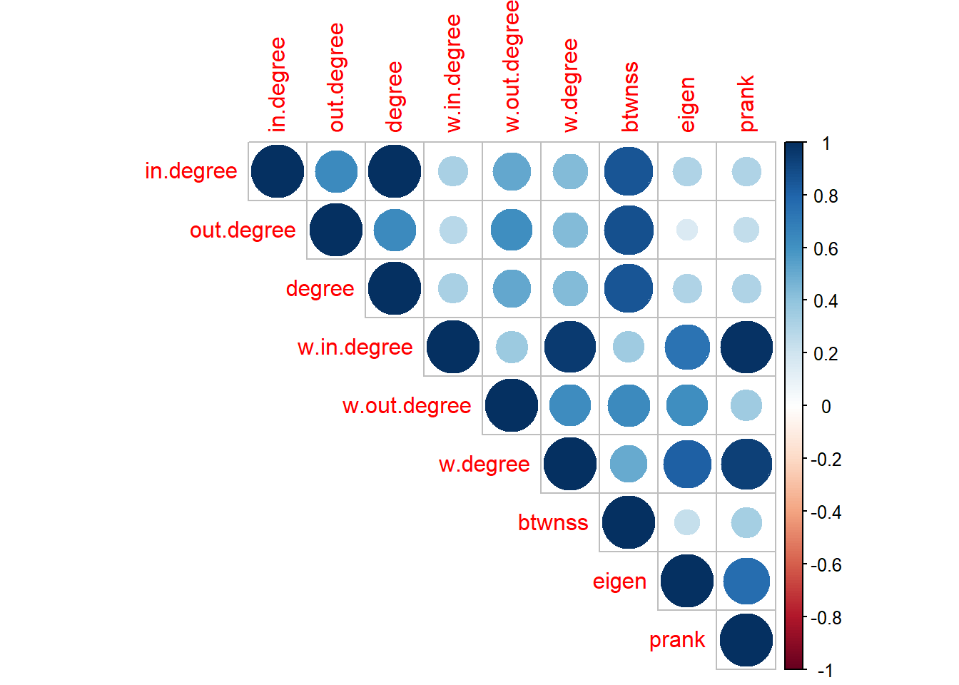

Question: Discuss the differences between the different centrality measures in the context of the commuting network.

Community detection

To begin with, we need to convert our network to an undirected one, as the fast_greedy algorithm we are using can only be applied to such networks.

net.all.und <- as.undirected(net.all,
                             mode=c("mutual"),
                             edge.attr.comb = igraph_opt("edge.attr.comb"))

communities.net.all <- cluster_fast_greedy(net.all.und)

# This provides a summary of the community algorithm:
print(communities.net.all)

IGRAPH clustering fast greedy, groups: 11, mod: 0.69
+ groups:
  $`1`
   [1] "E41000033" "E41000034" "E41000035" "E41000098" "E41000100" "E41000101"
   [7] "E41000102" "E41000104" "E41000106" "E41000107" "E41000127" "E41000130"
  [13] "E41000137" "E41000138" "E41000139" "E41000140" "E41000141" "E41000142"
  [19] "E41000143" "E41000144" "E41000145" "E41000146" "E41000147" "E41000148"
  [25] "E41000228" "E41000229" "E41000231" "E41000232" "E41000233" "E41000234"
  [31] "E41000236" "E41000293" "E41000294" "E41000295" "E41000296" "E41000297"
  [37] "E41000298" "E41000299" "E41000300" "E41000301" "E41000302" "E41000303"
  [43] "E41000304" "E41000305" "E41000306" "E41000307" "E41000308" "E41000309"
  [49] "E41000310" "E41000311" "E41000312" "E41000313" "E41000314" "E41000315"
  + ... omitted several groups/vertices

# To see how many communities we have, run the below:
length(communities.net.all)

[1] 11

# And these are the community sizes:
sizes(communities.net.all)

Community sizes
 1  2  3  4  5  6  7  8  9 10 11 
63 46 29 31 16 47 27 14 29 22 22 

# Now, let's create a new object with the community membership
#communities.net.all_membership <- membership(communities.net.all)

# And convert it to a data.frame

communities.net.all_membership <- membership(communities.net.all) %>%
  unclass %>%                          # we first need to unclass the object
  as.data.frame %>%                    # we convert it to a dataframe
  rename(community = ".") %>%          # rename the community column
  rownames_to_column("cmlad11cd") %>%  # we 'move' the rownames to a
                                       # new column in order to do a merge below
  left_join(la.names) %>%              # and now we can merge it with the LA names
  arrange(community) %>%               # arrange based on the community membership
  glimpse()

Rows: 346
Columns: 3
$ cmlad11cd <chr> "E41000033", "E41000034", "E41000035", "E41000098", "E410001…
$ community <dbl> 1, 1, 1, 1, 1, 1, 1, 1, 1, 1, 1, 1, 1, 1, 1, 1, 1, 1, 1, 1, …
$ cmlad11nm <chr> "Southend-on-Sea", "Thurrock", "Medway", "Basildon", "Brentw…

# this is just a test to see if the `left_join` led to any NAs
sapply(communities.net.all_membership, function(x) sum(is.na(x)))

cmlad11cd community cmlad11nm 
        0         0         0 

Let’s try now to map our output. We need the local authorities shape file we have already loaded.

# First we merge the `la` object with the community membership
la <- merge(la, communities.net.all_membership, by = "cmlad11cd")
# Please note that I used base R for the above. I could have easily used the dplyr
# equivalent. Which function would this be?

# just a check to see how the merge worked
sapply(la, function(x) sum(is.na(x))) 

    cmlad11cd      OBJECTID   cmlad11nm.x    cmlad11nmw   Shape__Area 
            0             0             0             0             0 
Shape__Length      GlobalID     community   cmlad11nm.y      geometry 
            0             0             0             0             0 

# And this is our map
ggplot(la, aes(fill = as.factor(community))) + 
  geom_sf() +
  ggtitle("Communities using the 'fast and greedy' algorithm")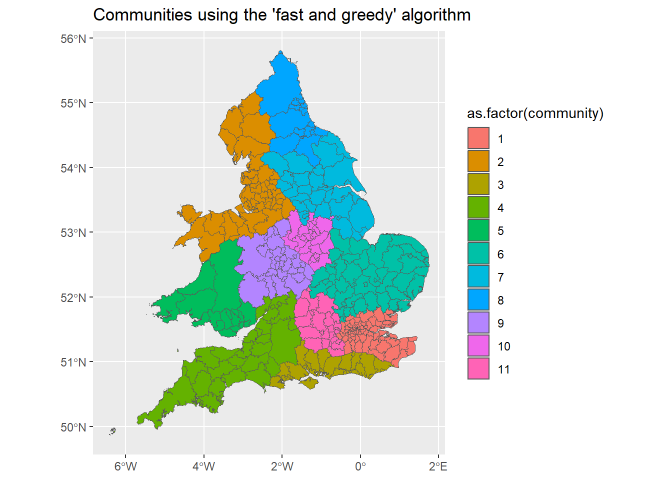

Question: What do you think about the output? Can we learn anything? Can you try different community algorithms? Check igraph’s manual and Javed et al (2018)

Network Visualisation

The below chunks of code offer some intro to plotting network data. Have a look to see how the code works.

plot(net.all, # the graph to be plotted
     layout=layout.fruchterman.reingold, # the layout method. see the igraph documentation for details
     main='My first graph in R', # specifies the title
     vertex.label.dist=0.5, # puts the name labels slightly off the dots
     vertex.frame.color='blue', # the colour of the border of the dots
     vertex.label.color='black', # the colour of the name labels
     vertex.label.font=2, # the font of the name labels
     vertex.label=V(net.all)$id, # specifies the labels of the vertices. in this case the 'name' attribute is used
     vertex.label.cex=.5,   # specifies the size of the font of the labels. can also be made to vary
     edge.arrow.size=0.1) # specifies the arrow size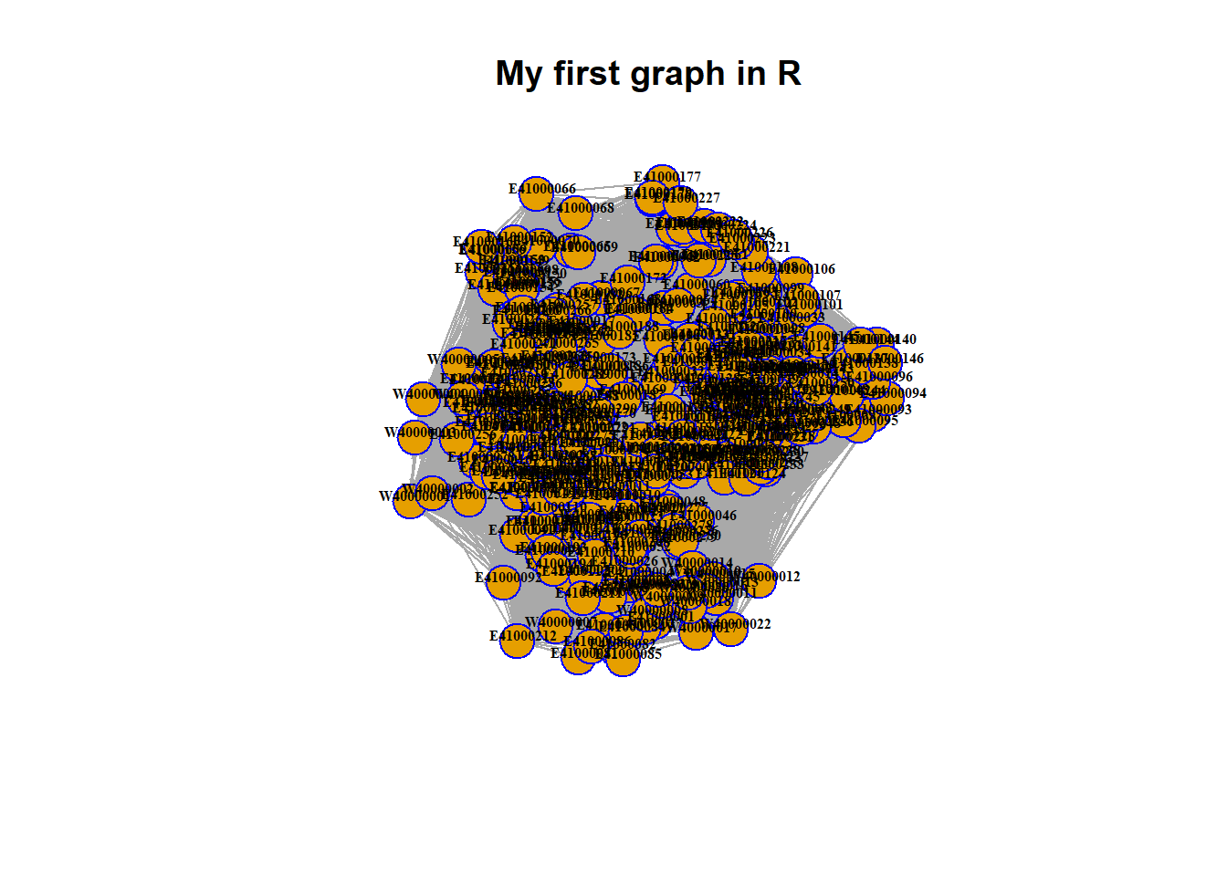

Not a very nice outcome :( Let’s remove some information

plot(net.all, # the graph to be plotted
     layout=layout.fruchterman.reingold, # the layout method. see the igraph documentation for details
     main='My second graph in R',   # specifies the title
     vertex.frame.color='blue', # the colour of the border of the dots
     vertex.label.font=2,   # the font of the name labels
     vertex.label=NA,   # no labels for the vertices
     edge.arrow.size=0, # specifies the arrow size
     vertex.size=5) # vertex size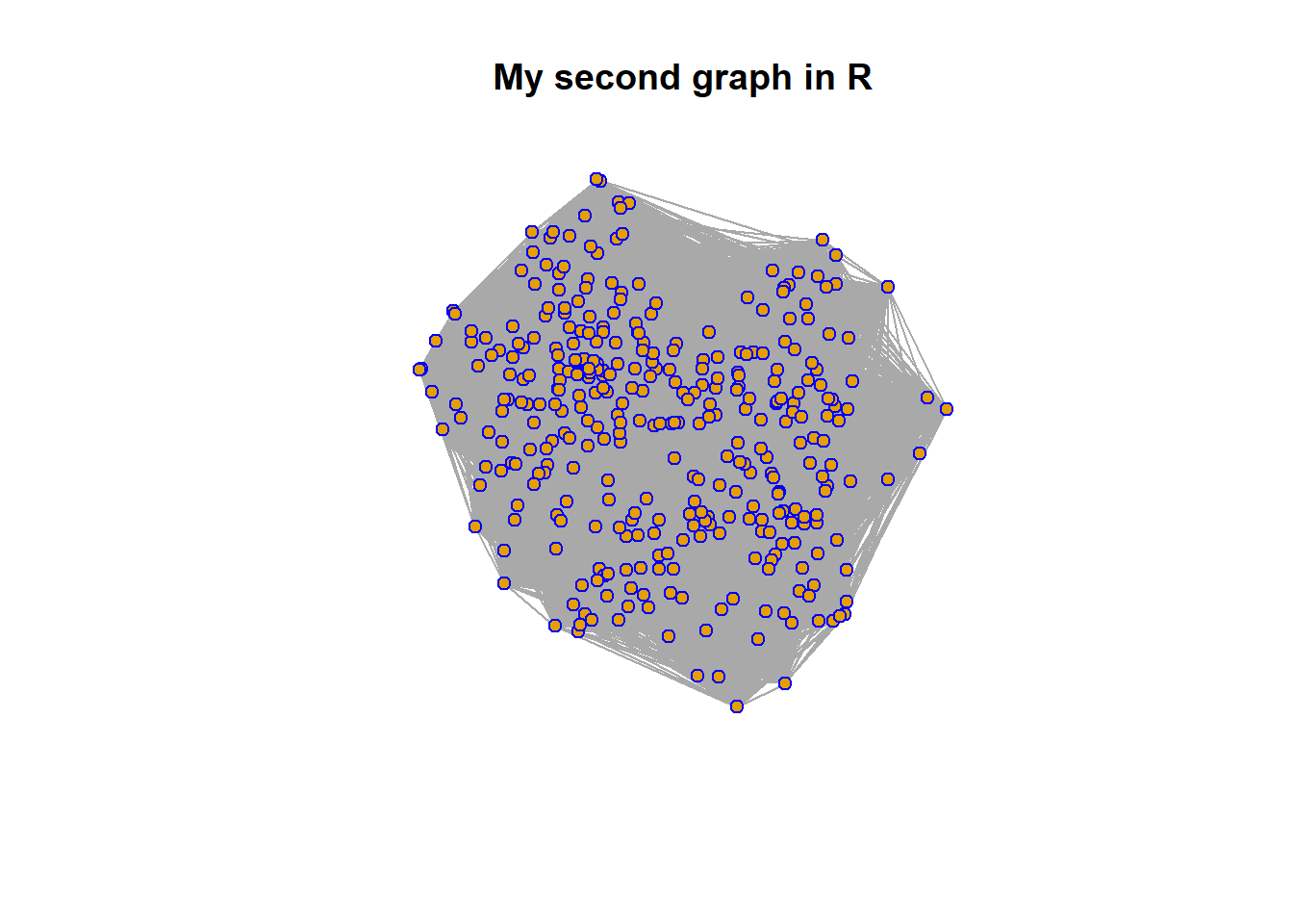

Let’s try to only plot nodes with high weighted degree centrality.

# The below gives us the 90th percentile:
q <- quantile(strength(net.all), .9)

# Then, we create a network with the nodes we DON'T want to plot. In this case the lowest 90%
low_nodes <- V(net.all)[strength(net.all) < q] # 108659 is the 90% percentile. Feel free to play with different numbers

# And this is the network with the 10% of the most central nodes
net.all.central <- delete.vertices(net.all, low_nodes)

# The below uses the node degree centrality to plot the node size.
# Pay attention to the 0.0001 factor.

plot(net.all.central, # the graph to be plotted
     layout=layout.fruchterman.reingold, # the layout method. see the igraph documentation for details
     main='My third graph in R', # specifies the title
     vertex.frame.color='blue', # the colour of the border of the dots
     vertex.label.font=2,   # the font of the name labels
     vertex.label=V(net.all.central)$id, # no labels for the vertices
     vertex.label.font=1, # the font type of the name labels (1 plain, 2 bold, 3, italic, 4 bold italic, 5 symbol)
     vertex.label.cex=.5,   # specifies the size of the font of the labels. can also be made to vary
     edge.arrow.size=0, # specifies the arrow size
     vertex.size=strength(net.all.central)*0.0001) # defines the node size based on weighted degree centrality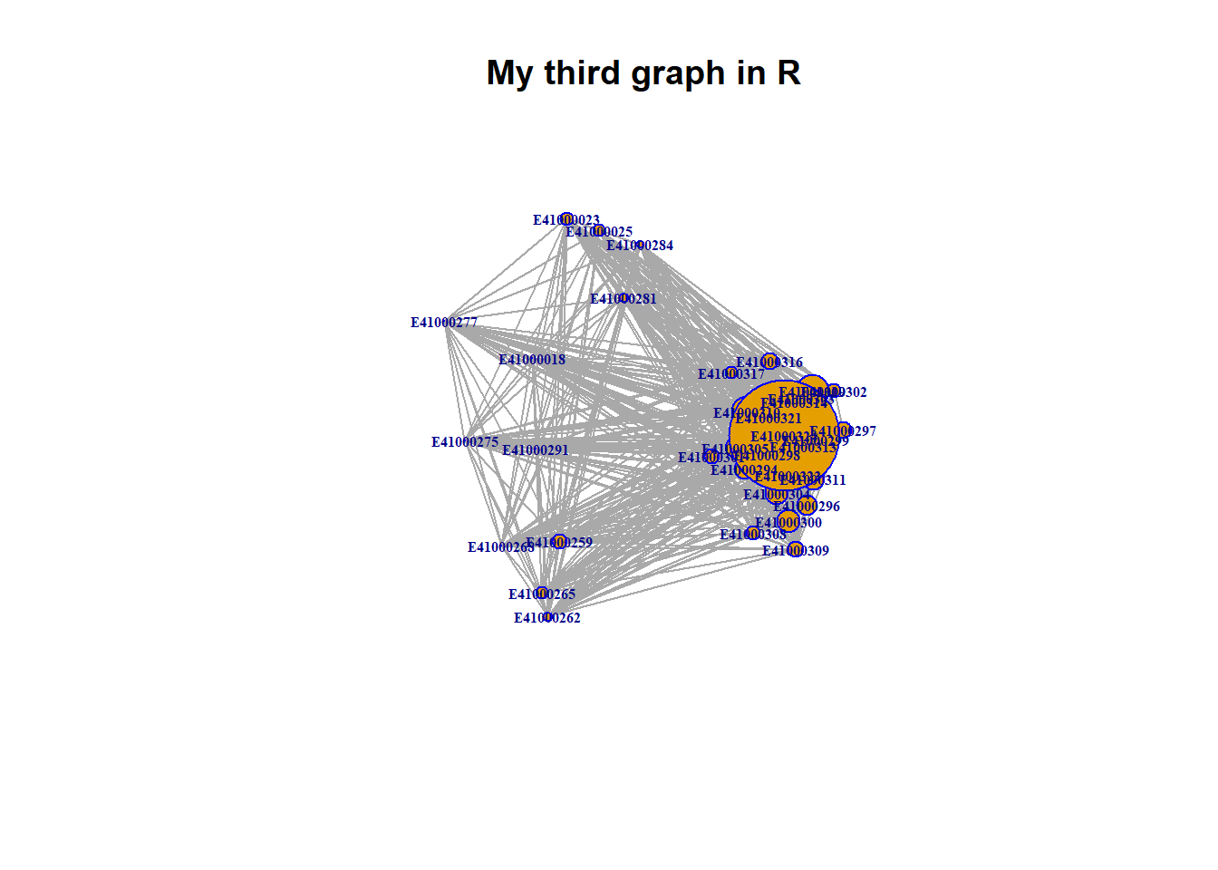

Not very nice either…

For the next time:

1. spend some time browsing the igraph’s manual,

2. search for code online to plot large netwoks in R using igraph, and

3. use the following tutorials

• netVizR (the data can be found here under the ‘Network Visualization in R’ section

• edge-bundling

in order to produce more meaningful network visualisations of the UK commuting network.

I am interesting in one or multiple plots with:

• all or a subset of the nodes and edges. How could you select such a subset?

• the communities you detected.

• varying size of nodes based on a centrality measure. Again, you can decide to plot a subset of the network based on some network characteristics.

• an appropriate to the network layout.

Mapping

Until now we focused mostly on the topology of the network and we ignored its spatial dimension. However, this is an important attribute of the commuting network and we should necessarily consider it and incorporate it in our analysis. To begin with we will map these commuting flows. Bare in mind that this is not a trivial process as, in essence, we need to attach the geographical coordinates to the network nodes and plot the network based on these coordinates. Given the size of our network this might be computationally expensive. It is also challenging to create a meaningful map given the size of the network.

The local authorities spatial object is necessary in order to use the od2line() function from the stplanr package. This is a very useful function transforms origin to destination (OD) tables to linear spatial objects. In order for this function to work we need the above spatial object with the zones of the origin and destination flows. Importantly it needs to only include the zone codes (i.e. the local authority codes), which should match with the origin and destination codes.This is the la spatial object of the local authorities in England and Wales, which has already been loaded in R.

The below code just plots the boundaries of local authorities.

ggplot(la) + 
  geom_sf() +
  ggtitle("Local authorities")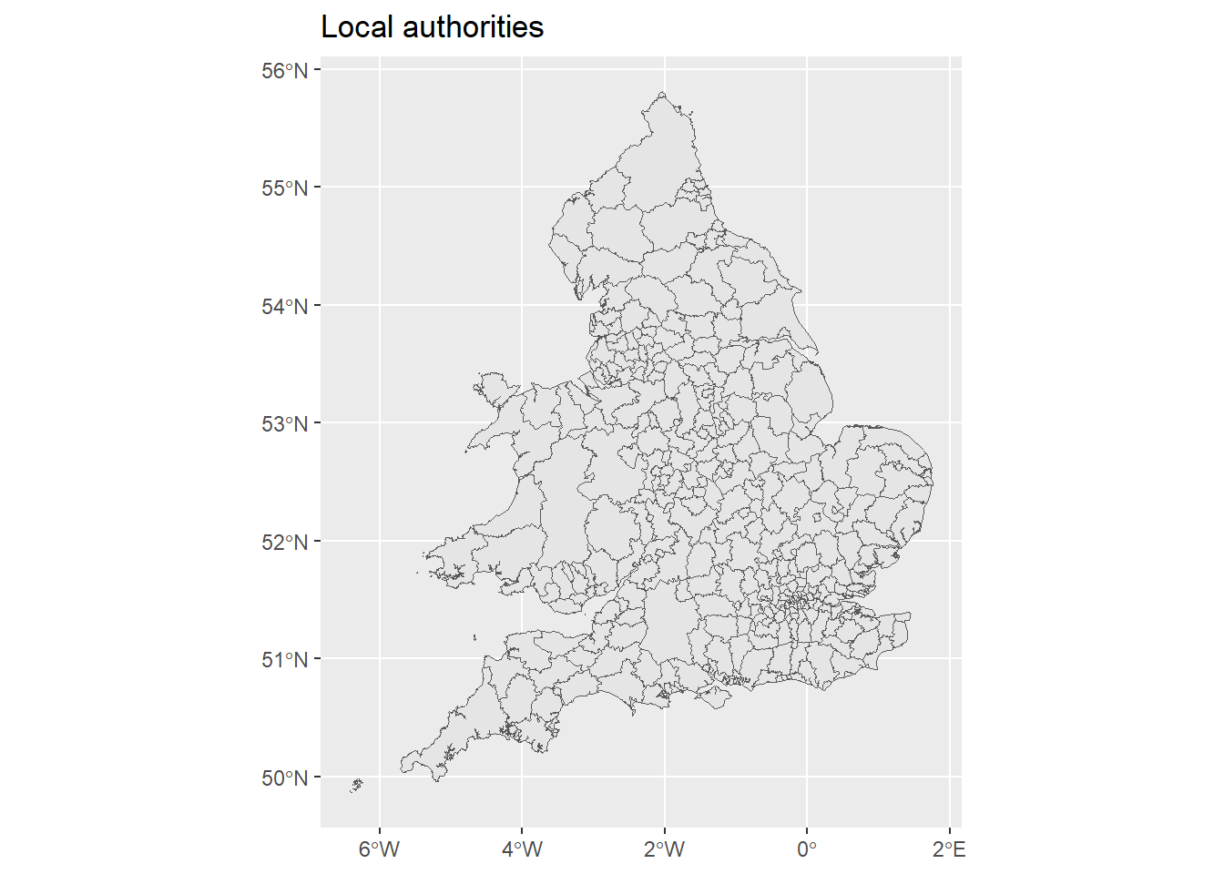

Now let’s do some clean-up of the commuting.all data frame in order to convert it to a spatial object using the od2line() function.

# We start by plotting a histogram of the data. We are using ggplot() as the output
# is nicer, but the simpler hist() could also be used

options(scipen=999) # It prevents R from using scientific notation for numbers
ggplot(commuting.all,
       aes(x=weight)) +
  geom_histogram() +
  geom_vline(aes(xintercept=mean(weight)), # This line of code adds a vertical line to represent the mean
             color="blue", linetype="dashed", size=1)

Warning: Using `size` aesthetic for lines was deprecated in ggplot2 3.4.0.
ℹ Please use `linewidth` instead.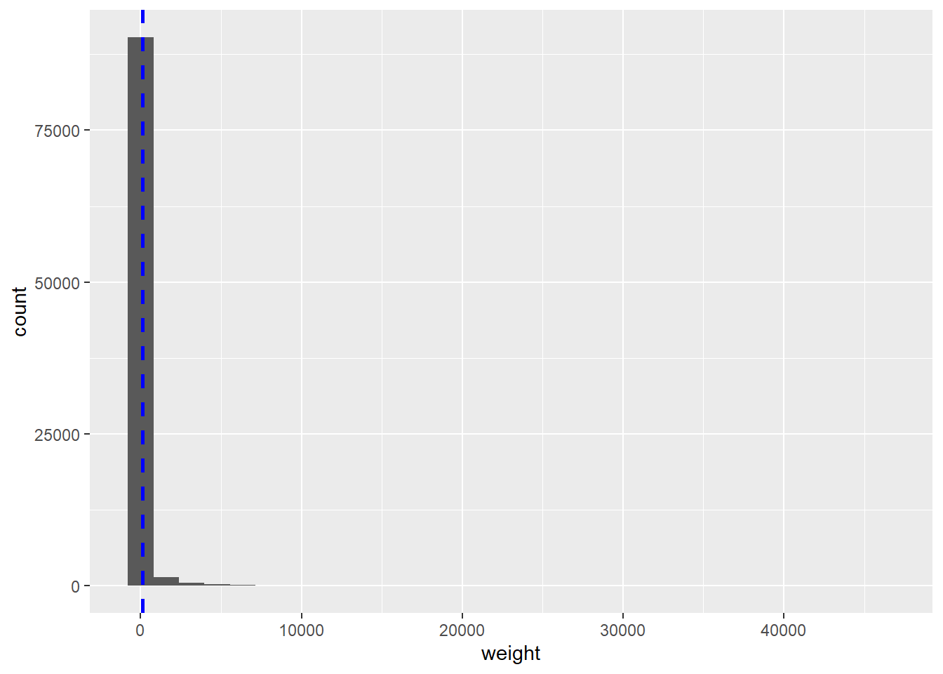

As you can see the flow data is very skewed. So, let’s truncate the data and plot a histogram for flows between origin and destinations will less than 1000 people.

ggplot(commuting.all[commuting.all$weight < 1000,],
       aes(x=weight)) +
  geom_histogram() +
  geom_vline(aes(xintercept=mean(weight)),
             color="blue",
             linetype="dashed",
             size=1)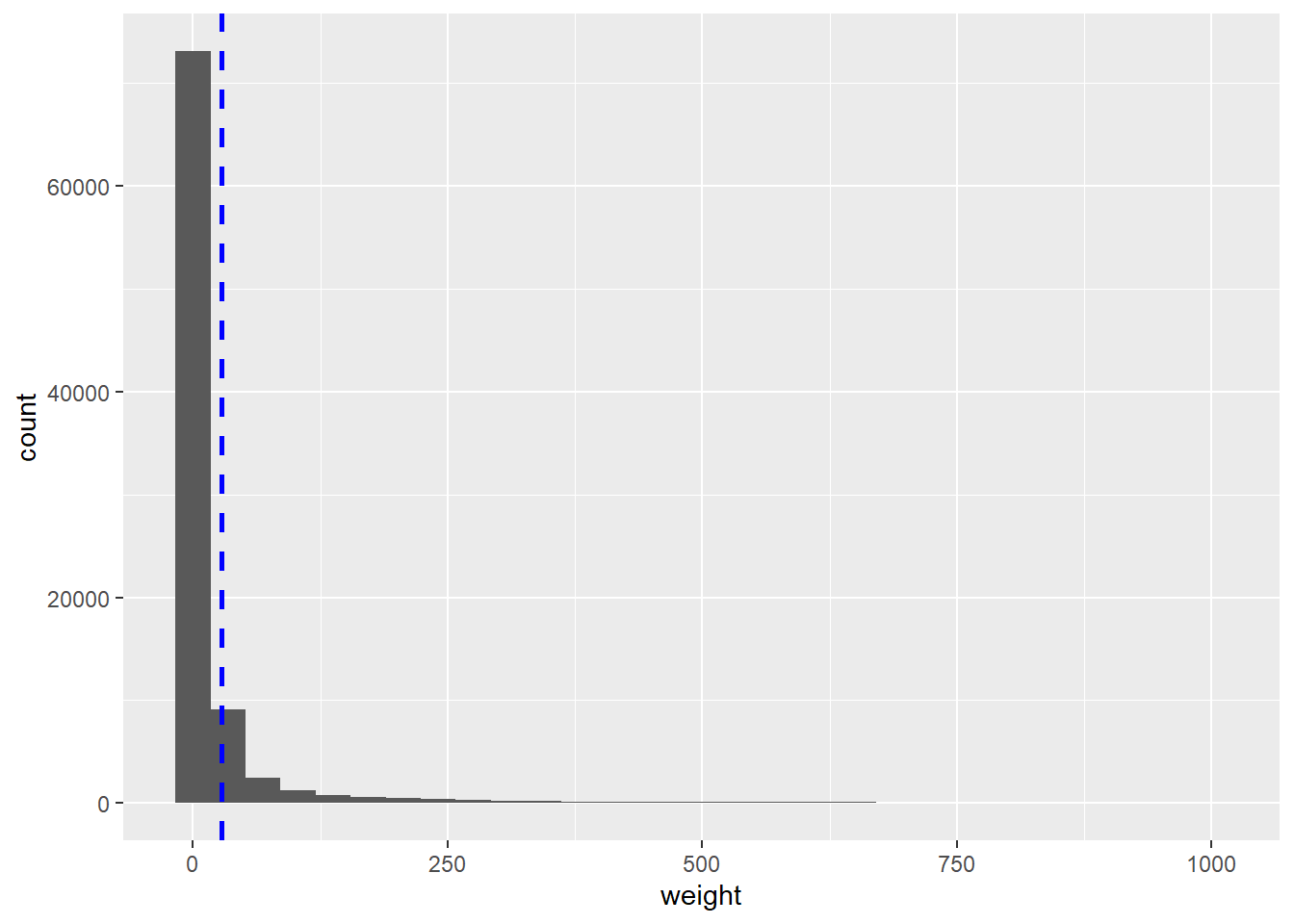

There is a very large number of local authority pairs with very few people commuting between these OD pairs. So, in order to decrease the data and the mapping complexity we will keep only the OD pairs with more than 5 commuters.

commuting.all.truncated <- commuting.all %>% 
  filter(weight > 5) %>% 
  glimpse()

Rows: 41,659
Columns: 3
$ o      <chr> "E41000001", "E41000001", "E41000001", "E41000001", "E41000001"…
$ d      <chr> "E41000002", "E41000003", "E41000004", "E41000005", "E41000010"…
$ weight <dbl> 1591, 534, 3865, 433, 8, 24, 6, 30, 6, 6, 10, 8, 6, 7, 7, 7, 9,…

Question: How many lines did we filter out?

The next chunk of code converts the origin-destination table to a spatial object using the corresponding zones spatial object (la) that we have already loaded.

# od2line() has some strict requirement regarding data structure. 
# Check ?od2line
# Therefore, we kept only the local authority code and name.
# The actual requirement is to have the the zone code as the 
# first column of the zone object. 
# If you remember, we run the following when we loaded the la object: 
# la.names <- as.data.frame(la) %>% 
#   select(cmlad11cd, cmlad11nm) # all we need is the LA names and codes

travel_network <- od2line(flow = commuting.all.truncated, 
                          zones = la)

# Just to see the class of the new spatial object
class(travel_network)

[1] "sf"         "data.frame"

plot(travel_network)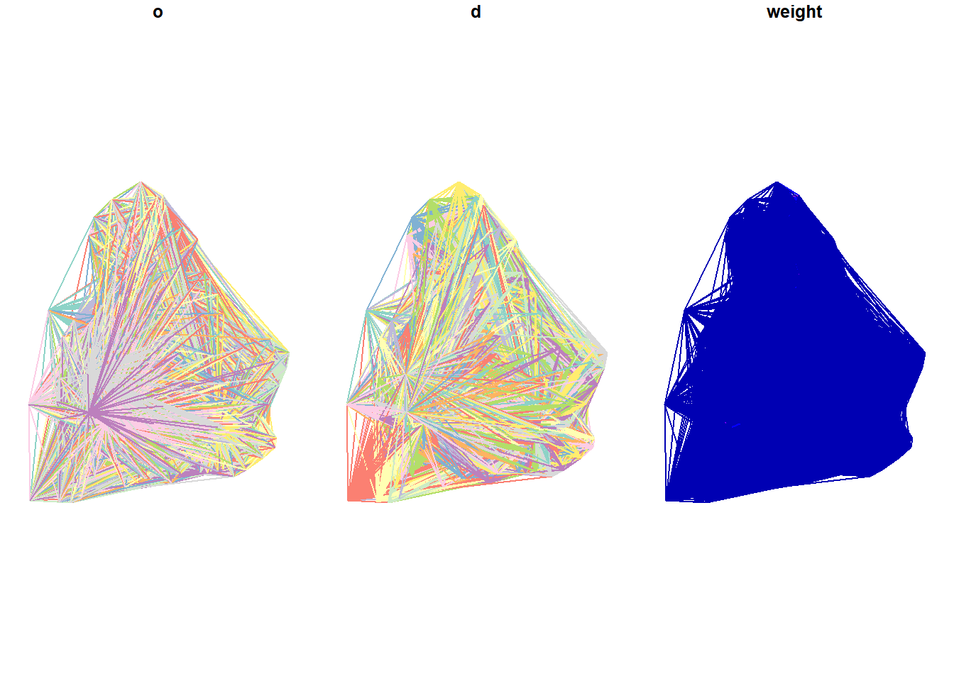

This is a naive plot of the spatial network. We can guess the shape of England and Wales, but this is like a hairball network and far from being useful. In order to produce a more useful visualisation we will employ the leaflet package, which produces interactive maps using JaveScript Libraries.

# this is the colour pallet we are going to use based on 5 quantiles
Flow_pal <- colorQuantile("YlOrBr", domain = travel_network$weight, n=5)

leaflet() %>%
  addTiles() %>%
  addPolylines(
    data = travel_network,
    weight = .1,
    color = ~Flow_pal(weight),
    opacity = .6) %>%
    addLegend("topright",
              pal = Flow_pal,
              values = travel_network$weight,
              title = "Commuting flows in 2011")

Let’s try now to create an interactive map showing only the flows originating from Bristol and Birmingham.

# To begin with let's find out the local authority codes for Bristol and Birmingham
# Look up the grep() function. Very useful!
la.names[grep("Bristol", la.names$cmlad11nm),]

   cmlad11cd        cmlad11nm
23 E41000023 Bristol, City of

la.names[grep("Birmingham", la.names$cmlad11nm),]

    cmlad11cd  cmlad11nm
281 E41000281 Birmingham

# These are E41000023 and E41000281 respectively.

# Next we will create the 'groups' of local authorities
travel_network$la.groups = "Rest"
travel_network$la.groups[travel_network$o == "E41000023"] = "Bristol"
travel_network$la.groups[travel_network$o == "E41000281"] = "Birmingham"

leaflet() %>%
  addTiles() %>%
  addPolylines(
    data = travel_network,
    weight = 1, # Notice the different value for better visual effect when zoom in
    color = ~Flow_pal(weight),
    opacity = .8, # as above
    group = travel_network$la.groups) %>%
  addLayersControl(
    position = "bottomleft",
    overlayGroups = unique(travel_network$la.groups),
    options = layersControlOptions(
      collapsed = FALSE)) %>%
  addLegend("topright",
          pal = Flow_pal,
          values = travel_network$weight,
          title = "Commuting flows in 2011")