Network models in practice

Setup

Pay attention on the packages sand and igraphdata. The first one contains all the different network datasets used by (Kolaczyk and Csárdi 2020). Then, the second one contain network data to be used together with the igraph package. More information can be found here and here. Feel free to explore these network data on your own time.

library(tidyverse)
library(igraph)

library(sand)       
library(igraphdata)

Aims of the practical

• Simulate network models

• Analyse their key attributes

• Compare them

igraph enables us to generate networks based on some of the some key network models we discussed. I list below some of these functions:

• sample_gnp()

• sample_smallworld()

• sample_pa()

Go to igraph’s webpage and familiarise yourselves with the syntax of these functions.

Task: Create three networks using these three functions with, let’s say, (n = 500) nodes each.

Visualise and compare these networks.

Importantly, just before you generate a network with one of the above three functions you will need to define a random seed for reproducibility reasons, e.g. set.seed(55).

Question: Without defining a random seed, generate a network as per the above, run some type of quick analysis about this network and then repeat the code by generating a second network with the exact same characteristics. Run the same analysis for the second network. Are the results the same?

Why do we need to define the random seed ?

Examples of modelled networks

sample_gnp(n = 500, p = 0.02) %>% 
  plot(layout=layout_in_circle, vertex.label=NA)

sample_pa(n = 500, directed=FALSE) %>% 
  plot(layout=layout_in_circle, vertex.label=NA)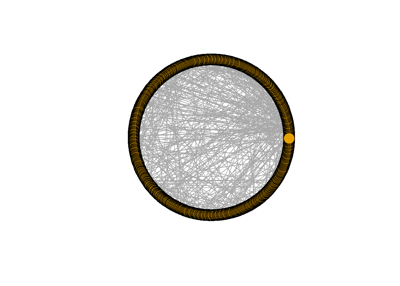

sample_smallworld(dim = 1, size = 500, nei = 5, p = 0.05) %>% 
  plot(layout=layout_in_circle, vertex.label=NA)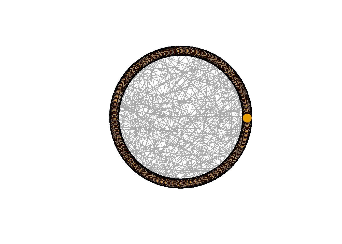

make_lattice(dim =1, length = 100, nei = 5) %>% 
  plot(vertex.label=NA)

Challenge 1: Think about the commuting datasets you used in the past tutorials. Is the commuters network Small World? Is it Scale-Free network?

Challenge 2: Can you demonstrate where would this graph sit on the scale between ranom and regular network using your knowledge centrality measures in I graph?

Challenge 3: Taking the commuters network or network of your choice, can you demonstrate the Bettencourt-West/Marshall’s law?

Challange 4 Taking the data and model from the challange 3, can you find the value of (/beta) (the exponent)? What does that value mean for your variables and the phenomena tehy represent?

Extra resources: - Network Analysis in R from Dai Shizuka - Statistical Analysis of Network Data with R - Awesom Network Analysis: list of useful R packages (and much more) - R Graph Gallery _ Static and dynamic network visualization with R from Katya Ognyanova

References

Kolaczyk, Eric D, and Gábor Csárdi. 2020. Statistical Analysis of Network Data with r. Second. Vol. 65. Springer.