Methods in transport geography
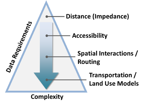
Source: Rodrigue (2020)
Spatial network from the graph theory perspective
 Source: Wu et al. (2019)
Spatial network from the graph theory perspective
Terminology
terminal = node = vertex
link = edge
Sub-graph - Loop (buckle)
More types of graphs
Planar graph vs Non-planar graph
Cycle, circuit
![]() Source: Rodrigue (2020)
Source: Rodrigue (2020)
Graph analysis
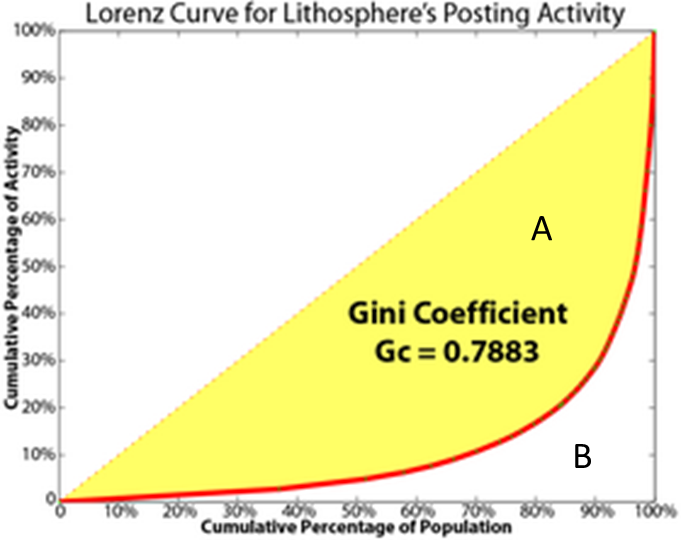
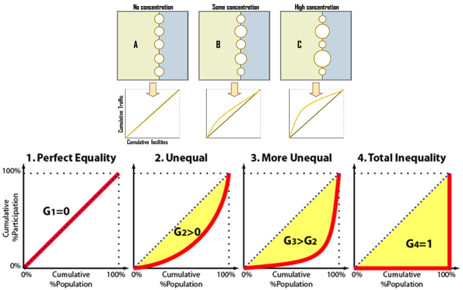
The Gini coefficient
Measure of dispersion often used as Inequality measure
- 0: perfect equality
- 1 :perfect inequality
Ordered X and Y, cumulative percentage
Mostly used for income inequalities, but can be more widely used
\(Gini = A / (A + B)\)
Source: Rodrigue (2020)
 Source: Rodrigue (2020)
 Source: Rodrigue (2020)
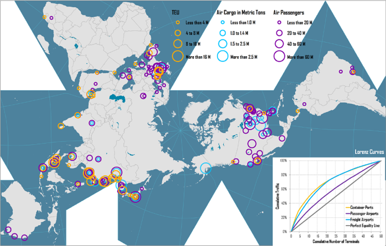
Example: measuring traffic concentration
Temporal variations of the Gini coefficient reflect changes in the comparative advantages of a location within the transport system
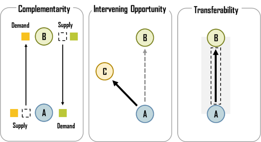
Spatial interactions and the gravity model
Conditions for spatial interaction to be materialised
 Source: Rodrigue (2020)
1. Calculate flows (naive)
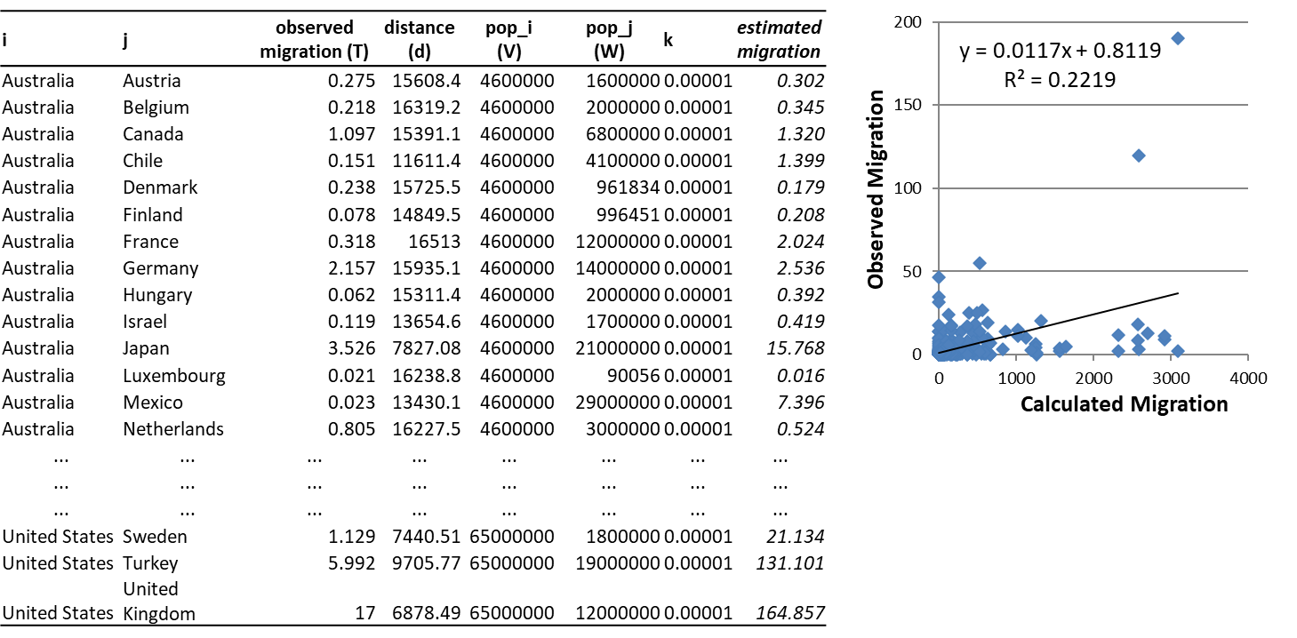
2. Estimate \(\lambda\), \(\alpha\), \(\beta\) and \(k\)

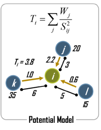
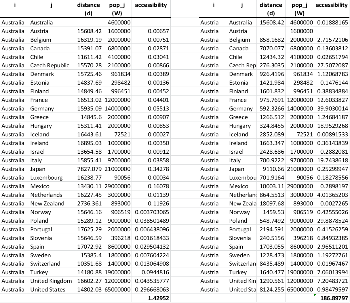
3. Estimate accessibility indicators
- \(Acc_{i} = \sum_j \frac{W_j}{d_{ij}^2}\)

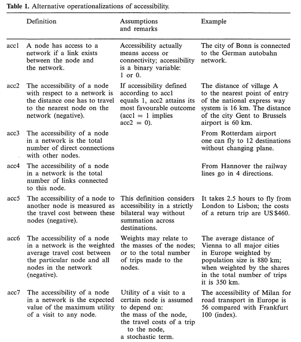
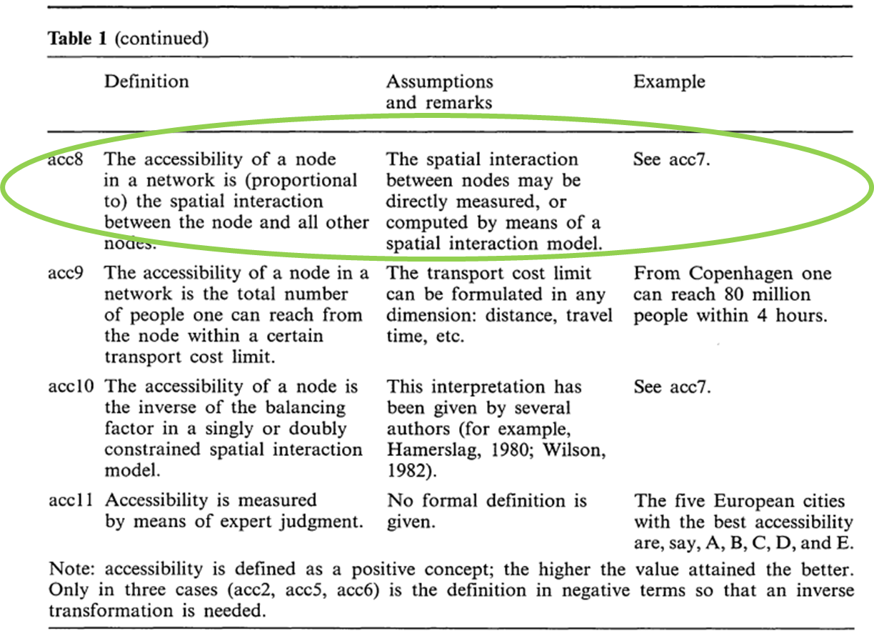
Accessibility of locations from routing perspective

Accessibility of locations from routing perspective

Vrabková, Ertingerová, and Kukuliač (2021)

Vrabková, Ertingerová, and Kukuliač (2021)