Methods in transport geography

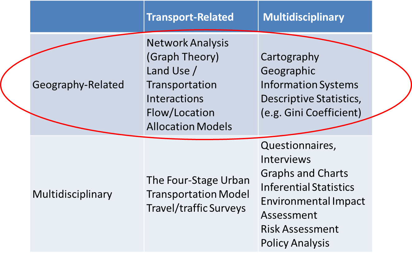
Transport geography: quantitative dimension

• Empirical data

• Data analytics

• Applied science: improve the efficiency of movements / spatial constraints

• Why in this unit?

Transport geography: key elements

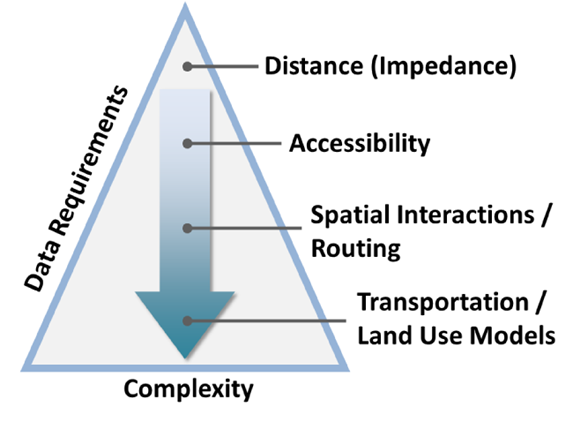
• Distance

• Accessibility: the capacity of a location to be reached by, or to reach different locations

• Spatial interaction: movement of people, freight or information between an origin and destination

• Transportation and land use models

Source: Rodrigue (2020)

Source: Rodrigue (2020)

Graph theory, aka network analysis

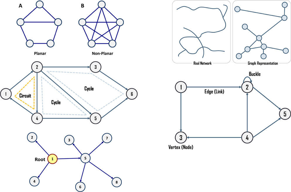
• Abstraction

• Represent the structure not the appearance

• Terminal = node

• Node (vertex)

• Link (edge)

• Sub-graph - Loop (buckle)

• Planar graph

• Non-planar graph

• Cycle, circuit

• Tree \((e = v-1)\)

Source: Rodrigue (2020)

Graph theory, aka network analysis

• \(\beta = e / v\), where \(e\) is the number of links & \(v\) the number of nodes

• \(Gamma\) AKA network density (number of liks / maximum number of links)

  • planar: \(\gamma = \frac{e}{3(v-2)}\)

  • non-planar: \(\gamma = \frac{2e}{v(v-1)}\)

Graph theory, aka network analysis

• Degree centrality

• Eccentricity: the distance from a given node to the farthest node from it in the network

• Shimbel index, or nodal accessibility, or Fareness (see Lecture 3

  • \(c_𝑖= \sum_j d_{ij}\)

  • This is a purely topological accessibility metric, remember this for later.

Closeness centrality (from Lecture 3)

• Which node has the shortest distance to other nodes

• Instead of focusing on the number of links, the focus turns to the network distances

• Different definitions:

• Closeness, \(c_{i} = 1/\sum_{j} d_{ij}\)

• Fareness, \(c_{i} = \sum_{j} d_{ij}\)

• igraph calculates closeness

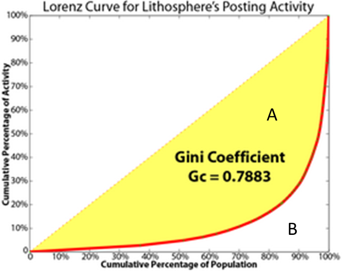
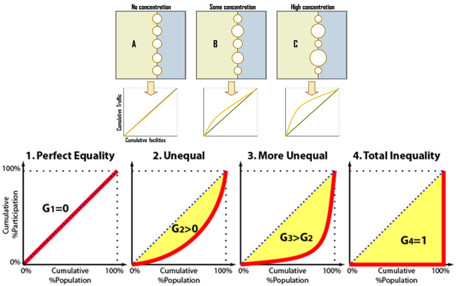
The Gini coefficient

• Inequality measure

  • 0: perfect equality
  • 1 :perfect inequality

• Ordered X and Y, cumulative percentage

• Mostly used for income inequalities, but can be more widely used

• \(Gini = A / (A + B)\)

Source: Rodrigue (2020)

Source: Rodrigue (2020)

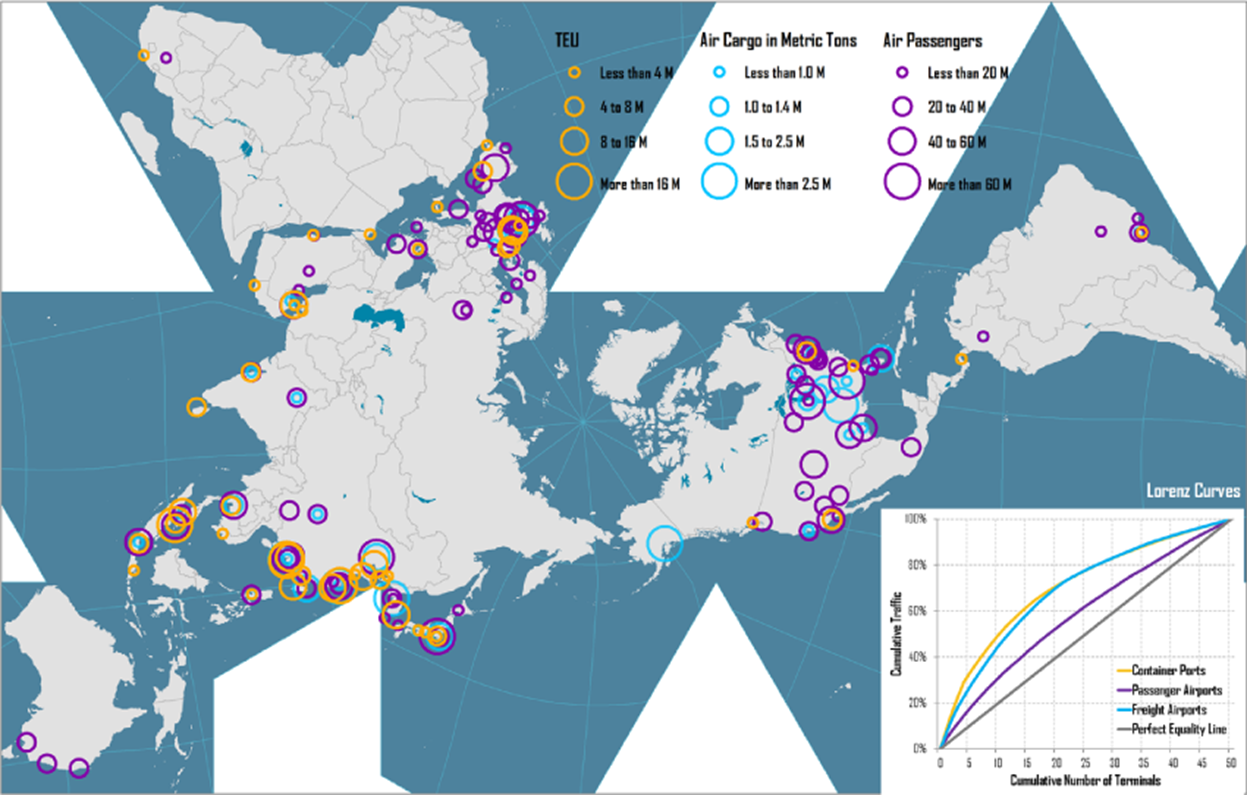Source: Rodrigue (2020)

The Location Quotient Coefficient

• Degree of concentration of a certain activities

• Very common for regional analysis too

• \(M_{ti}\) is the traffic of a merchandise \(t\) at a terminal \(i\)

• \(Mi\) is the traffic of all merchandise at a terminal \(i\)

• \(M_{t}\) is the total of all merchandises of type \(t\) for all terminals, and

• \(M\) is the total of all types of merchandises for all terminals

The Location Quotient Coefficient

\(LQ = \frac{\frac{M_{it}}{M_i}}{\frac{M_t}{M}}\)

• \(LQ <1\): traffic of merchandise \(t\) in terminal \(i\) is under-represented compared to the same merchandise in all terminals

• \(LQ = 1\) traffic of merchandise \(t\) in terminal \(i\) is proportional to its participation to total traffic

• \(LQ > 1\) traffic of merchandise \(t\) in a terminal \(i\) is preponderant in total traffic.

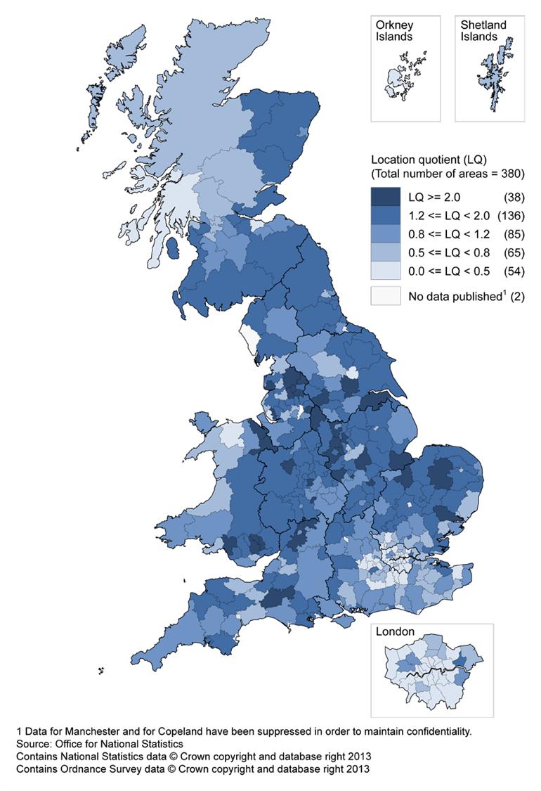
Employment in manufacturing sector

Source: ONS

Spatial interactions and the gravity model

• A spatial interaction is a realised movement of people, freight or information between an origin and a destination

• It is a transport demand/supply relationship expressed over geographical space.

Spatial interactions and the gravity model

Conditions for spatial interaction to be materialised

• Complementarity

• Intervening opportunity

• Transferability

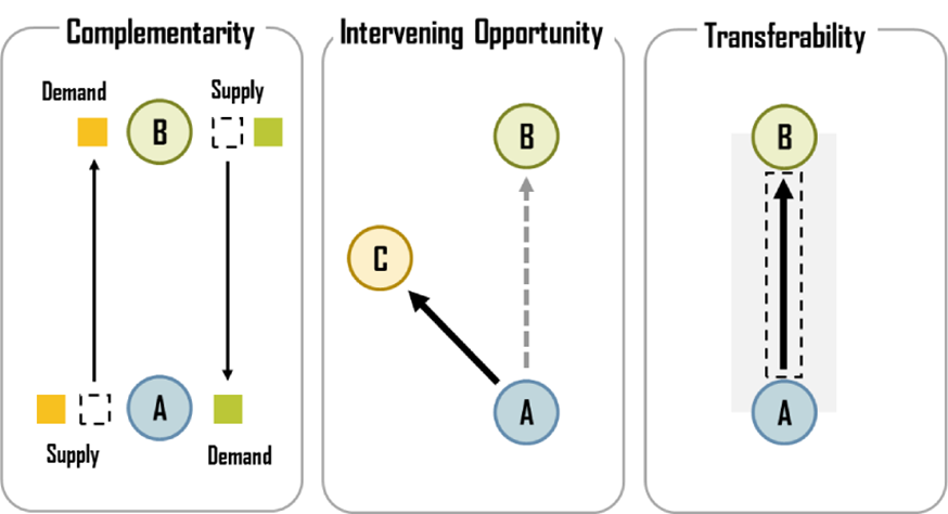Source: Rodrigue (2020)

Spatial interactions and the gravity model

• Origin/destination matrices

• Very large matrices

• Missing data/0s

• Estimation of flows

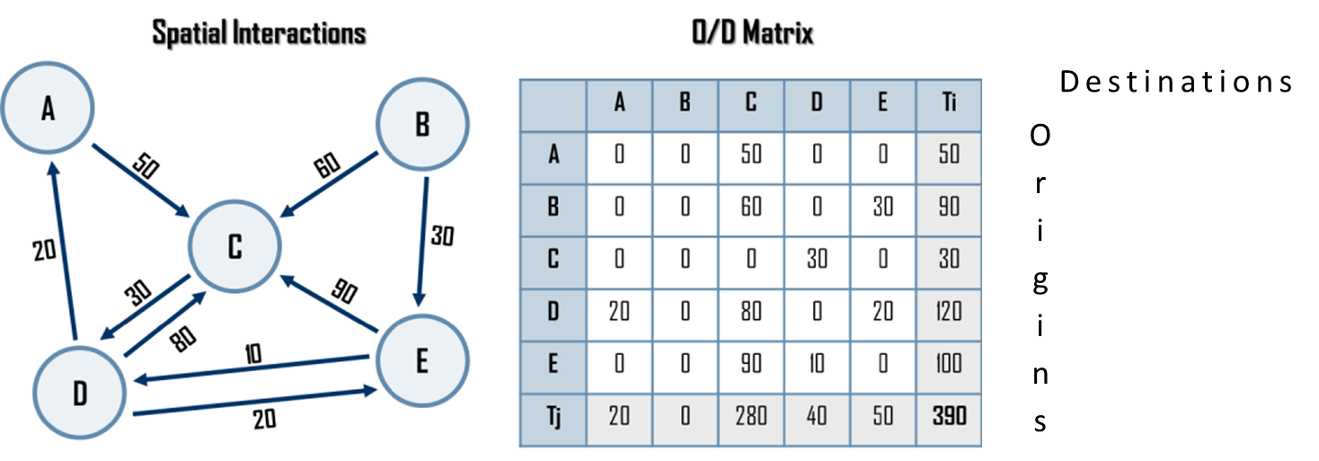
Spatial interactions and the gravity model

\(T_{ij} = f(V_i, W_j, S_{ij})\)

• Flows are a function of the attributes of the locations of origin, the attributes of the locations of destination and the friction of distance between the concerned origins and the destinations

Spatial interactions and the gravity model

\(T_{ij} = f(V_i, W_j, S_{ij})\)

• \(T_{ij}\): Interaction between location \(i\) (origin) and location \(j\) (destination)

• \(V_i\): Attributes of the location of origin \(i\) (e.g. population, number of jobs available, industrial output, GDP); push factors; the potential of origins

Spatial interactions and the gravity model

\(T_{ij} = f(V_i, W_j, S_{ij})\)

• \(W_j\): Attributes of the location of destination \(j\), pull factors; attractiveness of destinations

• \(S_{ij}\): Attributes of separation between \(i\) and \(j\) (e.g. distance, transport costs, or travel time); cost of overcoming the separation between origins and destinations

Spatial interactions and the gravity model

\(T_{ij} = k\frac{V_i^\lambda W_j^\alpha}{d_{ij}^\beta}\)

• \(\beta\): transport friction parameter

• \(\lambda\): Potential to generate movements

• \(\alpha\): Potential to attract movements

What can we do with this?

1. Calculate flows (naive)

\(T_{ij} = k\frac{V_i^\lambda W_j^\alpha}{d_{ij}^\beta}\)

• Known: \(V\), \(W\), and \(d\)

• Define: \(\lambda=1\), \(\alpha=1\), \(\beta=2\), and \(k=0.00001\)

• These are some standard values based on past empirical studies

• Big unknown: \(T\)

• Example from Tranos, Gheasi, and Nijkamp (2015)

1. Calculate flows (naive)

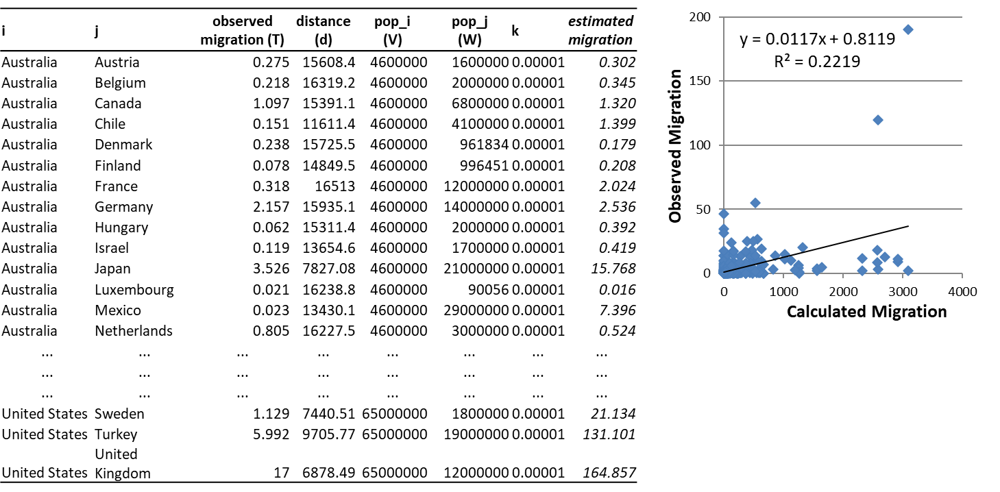
1. Calculate flows (naive)

• Fairly good estimation of reality for such an oversimplified model, but…

• … not good enough.

2. Estimate \(\lambda\), \(\alpha\), \(\beta\) and \(k\)

• Known: \(T\), \(V\), \(W\), \(d\) and \(k\)

• Estiamte: \(\lambda=1\), \(\alpha=1\), and \(\beta=2\)

• Why? To understand the effect of distance, pull and push factors

• How? Regression

2. Estimate \(\lambda\), \(\alpha\), \(\beta\) and \(k\)

• \(T_{ij} = k\frac{V_i^\lambda W_j^\alpha}{d_{ij}^\beta}\)

• Look up properties of logarithms, e.g. here

• \(T_{ij} = kV_i^\lambda W_j^\alpha d_{ij}^{-\beta}\)

• \(ln T_{ij} = ln (kV_i^\lambda W_j^\alpha d_{ij}^{-\beta})\)

• \(ln T_{ij} = lnk + lnV_i^\lambda + ln W_j^\alpha + lnd_{ij}^{-\beta}\)

• \(\color{red}{ln T_{ij}} = \color{blue}{lnk} + \lambda \color{green}{lnV_i} + \alpha \color{orange}{ln W_j} -\beta \color{purple}{lnd_{ij}}\)

• \(\color{red}{y} = \color{blue}{c} + \lambda \color{green}{x_1} + \alpha \color{orange}{x_2} + \beta \color{purple}{x_3}\)

• Multivariate linear regression

2. Estimate \(\lambda\), \(\alpha\), \(\beta\) and \(k\)

2. Estimate \(\lambda\), \(\alpha\), \(\beta\) and \(k\)

• \(c = lnk: -13.84\)

• \(\lambda = lnV_i: 0.727\)

• \(\alpha = lnW_j: 0.464\)

• \(\beta = lnd_{ij}: -0.624\)

• What did we learn?

• How can we use these coefficients

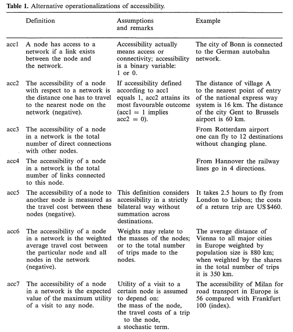
3. Estimate accessibility indicators

• The potential of opportunities for interaction

• Ease of spatial interaction

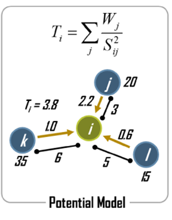
• Attractiveness of a node in a network taking into account the mass of other nodes and the costs to reach those nodes via the network

3. Estimate accessibility indicators

Different typologies (Holl 2007)

1. Network access

   • distance to access the network

   • travel opportunities

2. Travel cost measures

   • network access + distance/time travelled on the network

3. Market potential accessibility

   • destinations at greater distance provide diminishing opportunities

Source: Bruinsma and Rietveld (1998)

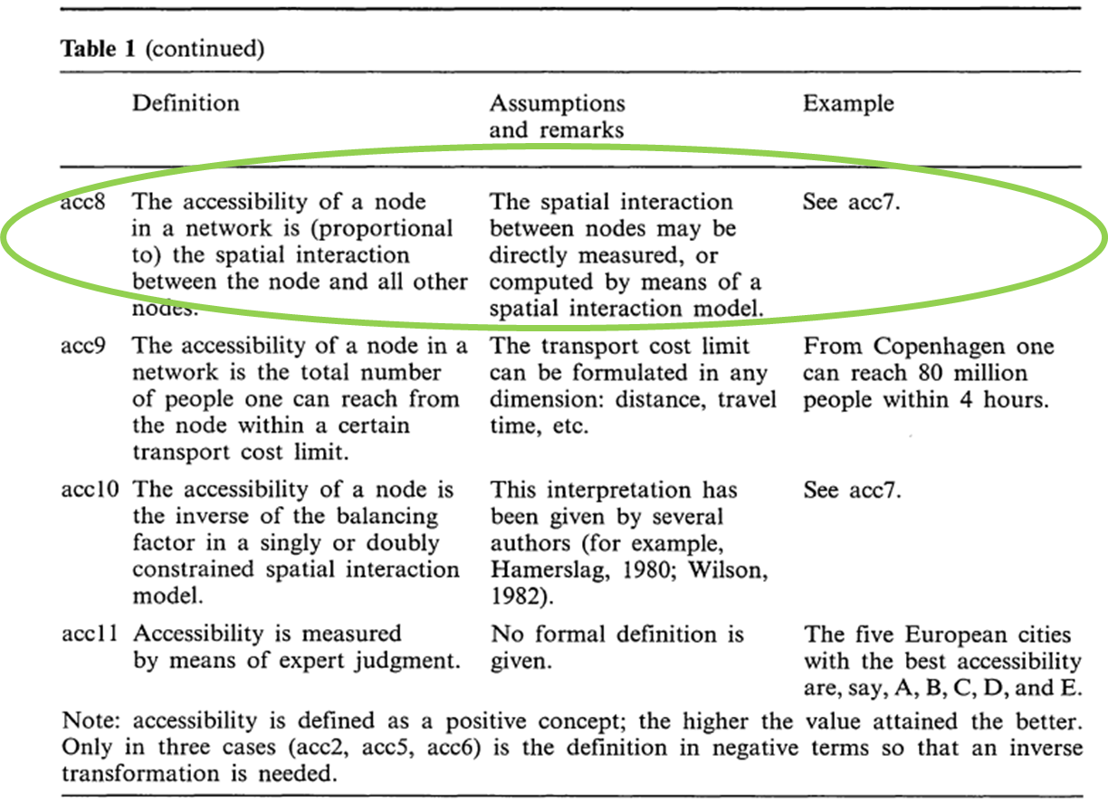
3. Estimate accessibility indicators

• \(Acc_{i} = \sum_j \frac{W_j}{d_{ij}^2}\)

Source:Rodrigue (2020)

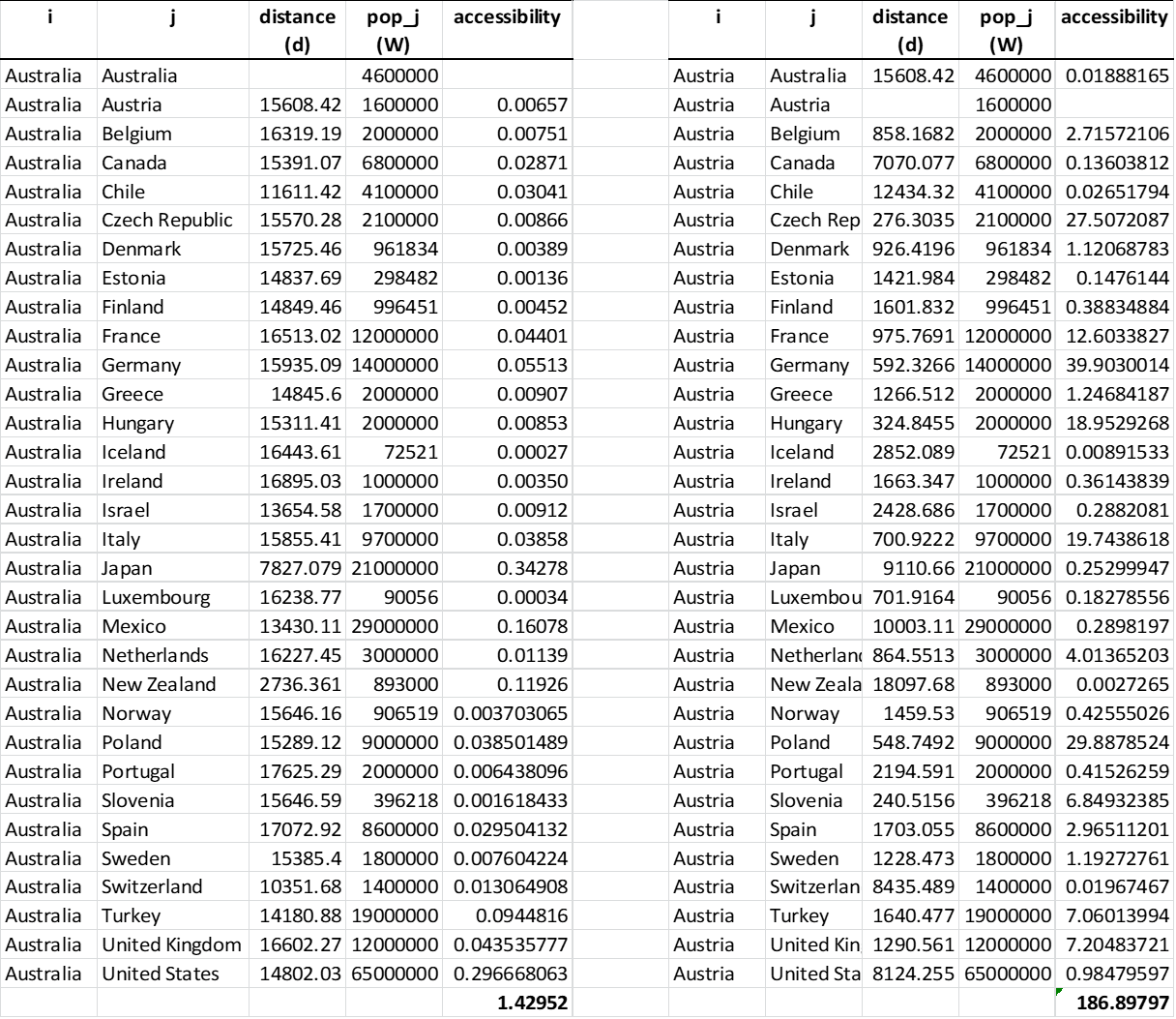
3. Estimate accessibility indicators

• Geographical indicator

• Spatial structure (e.g. distance) and economic activities (e.g. population)

• The potential for interaction

• Opportunities

References

Bruinsma, Frank, and Pieter Rietveld. 1998. “The Accessibility of European Cities: Theoretical Framework and Comparison of Approaches.” Environment and Planning A 30 (3): 499–521.

Holl, Adelheid. 2007. “Twenty Years of Accessibility Improvements. The Case of the Spanish Motorway Building Programme.” Journal of Transport Geography 15 (4): 286–97. https://doi.org/https://doi.org/10.1016/j.jtrangeo.2006.09.003.

Rodrigue, Jean-Paul. 2020. The Geography of Transport Systems. Routledge. https://transportgeography.org/.

Tranos, Emmanouil, Masood Gheasi, and Peter Nijkamp. 2015. “International Migration: A Global Complex Network.” Environment and Planning B: Planning and Design 42 (1): 4–22.